
My notes from the Machine Learning Course provided by Andrew Ng on Coursera
What is Machine Learning?
"The field of study that gives computers the ability to learn without being explicitly programmed"
~Arthur Samuel (1959)
“A computer program is said to learn from experience E with respect to some class of tasks T and performance measure P, if its performance at tasks in T, as measured by P, improves with experience E"
~Tom Mitchell (1998)
Supervised learning
- We know how the correct output should look like
- We know the relationship between the input and output
- Two types of supervised learning:
- Regression
- Classification
Regression
- Predict values based on labelled data
- Continuous valued output
Example: House size -> Sell prize
Classification
- Predict discrete valued label
Example: Email -> Spam or not
Binary or Binary Classification – group data in two types of label
Multi-class or Multinomial Classification – group data in more than two kinds of label
Unsupervised learning
- Have only dataset given (without labelled data)
- Algorithms finding structure in data
- No feedback based on the prediction results
- Two types of unsupervised learning:
- Clustering
- Non-clustering
Clustering
Example: Collection on 1 000 000 different genes and find in automatically group these genes into groups that are somehow similar or related by different variables, such as lifespan, location, roles, etc.
Non-clustering
Example: Cocktail Party Algorithm – allows to find structure in a chaotic environment
Supervised Learning vs Unsupervised Learning
- Supervised Learning will ALWAYS have an input-output pair
- Unsupervised Learning will have ONLY data with no label and will try to find some structure
Model Representation
x^{(i)}– input variable (input feature)y^{(i)}– output variable (target variable that we are trying to predict)x^{(i)},y^{(i)}– training examplex^{(i)},y^{(i)});ⅈ=1,…,m– training set- Function
h:X→Y– hypothesis, the output of the learning algorithm, whereh(x)is a good predictor fory

Regression -> if y is continuous
Classification – if y is a small set of discrete values
Regression Problem (Linear Regression)
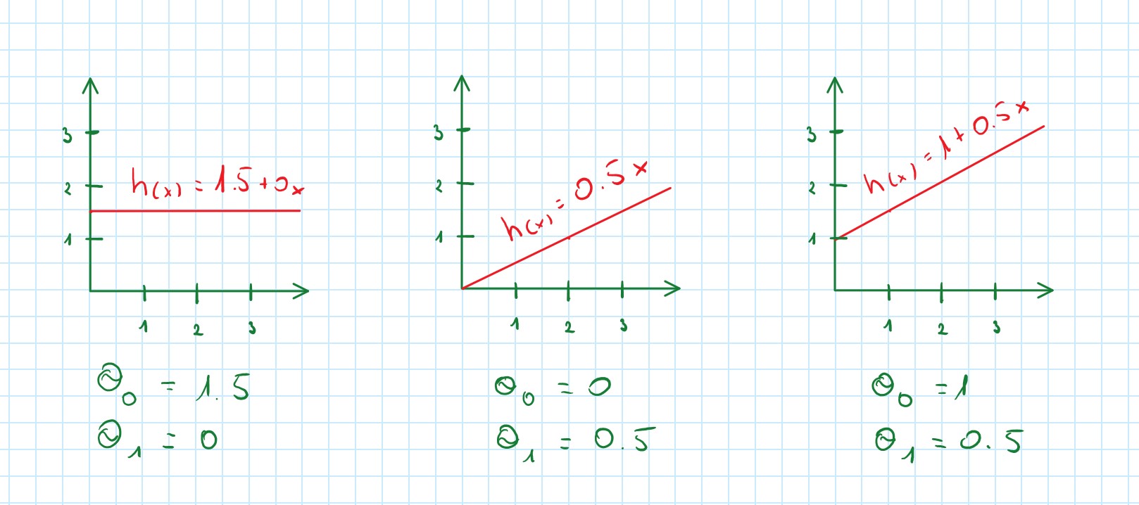
Linear Regression with one variable x and two parameters θ
h_θ (x)=θ_0+θ_1 x – linear function
Regression problem predict a continuous-valued label
Cost Function
The occurrence of Hypothesis Function can be measured by using Cost Function
- Hypothesis:
h_θ (x)=θ_0+θ_1 x - Parameters:
θ_0,θ_1 - Cost function:
J(θ_0,θ_1 )=\frac{1}{2m} \displaystyle\sum_{i=1}^m (h_θ (x_i )-y_i )^2 - Goal:
\frac{minimize}{θ_0,θ_1} J(θ_0,θ_1)
Other names for this J(θ_0,θ_1) cost function:
- Squared error function
- Mean squared error
Gradient descent
Finds local minimum for cost function J(θ_0,θ_1)
Gradient descent algorithm
repeat until convergence {
θ_j ≔ θ_j-α \frac{∂}{∂θ_0} J(θ_0,θ_1)
}
Parameter θ should be simultaneously updated at each iteration
Example:
temp0 ≔ θ_0-α \frac{∂}{∂θ_0} J(θ_0,θ_1)
temp1 ≔ θ_1-α \frac{∂}{∂θ_0} J(θ_0,θ_1)
θ_0 := temp0
θ_1 := temp1
Gradient Descent Intuition
- Finds local minimum
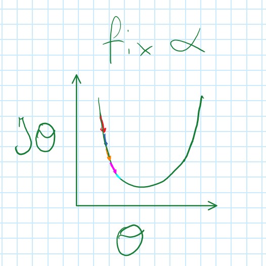
- Coverages to a local minimum with fixed α because derivative becomes smaller (baby steps)
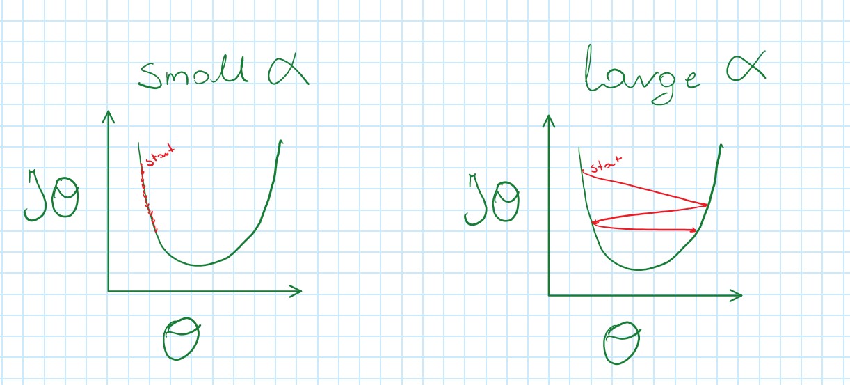
Learning Rate α
- If α is too small, Gradient Descent is slow
- If α is too large, Gradient Descent can overstep minimum and not coverage
Choosing a proper learning rate α in the beginning and stick to it at each iteration since Gradient Descent will automatically take smaller steps when approaching local minimum.
Gradient Descent for Linear Regression
Linear Regression with one variable
Gradient descent algorithm
repeat until convergence {
θ_j ≔ θ_j-α \frac{∂}{∂θ_0} J(θ_0,θ_1)
(for j=1 and j=0)
}
Linear Regression Model
h_θ (x)=θ_0+θ_1 x
J(θ_0,θ_1 )=\frac{1}{2m} \displaystyle\sum_{i=1}^m (h_θ (x_i )-y_i )^2
-
Calculate partial deviation $\frac{∂}{∂θ_0} J(θ_0,θ_1)$
\frac{∂}{∂θ_0}J(θ_0,θ_1 )=\frac{1}{2m} \displaystyle\sum_{i=1}^m (h_θ (x_i )-y_i )
\frac{∂}{∂θ_1}J(θ_0,θ_1 )=\frac{1}{2m} \displaystyle\sum_{i=1}^m ((h_θ (x_i )-y_i)x_i) -
So gradient descent becomes
repeat until convergence {
θ_0 := θ_0 - \alpha \frac{1}{m} \displaystyle\sum_{i=1}^m (h_θ (x^{(i)} )-y^{(i)})
θ_1 := θ_1 - \alpha \frac{1}{m} \displaystyle\sum_{i=1}^m (h_θ (x^{(i)} )-y^{(i)})x^{(i)}
} -
m=> size of the training set -
θ_0, θ_1=> constants that are changing simultaneously -
x_i, y_i=> values of the given training set
Gradient descent is called batch gradient if it needs to look at every example in the entire training set at each step
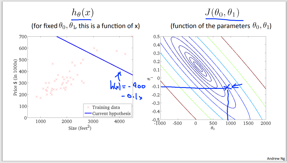
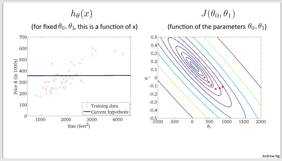
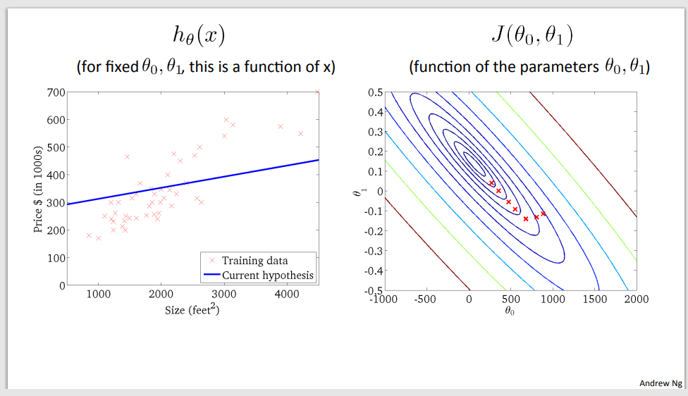
Example of gradient descent to minimalize cost function
Step 1
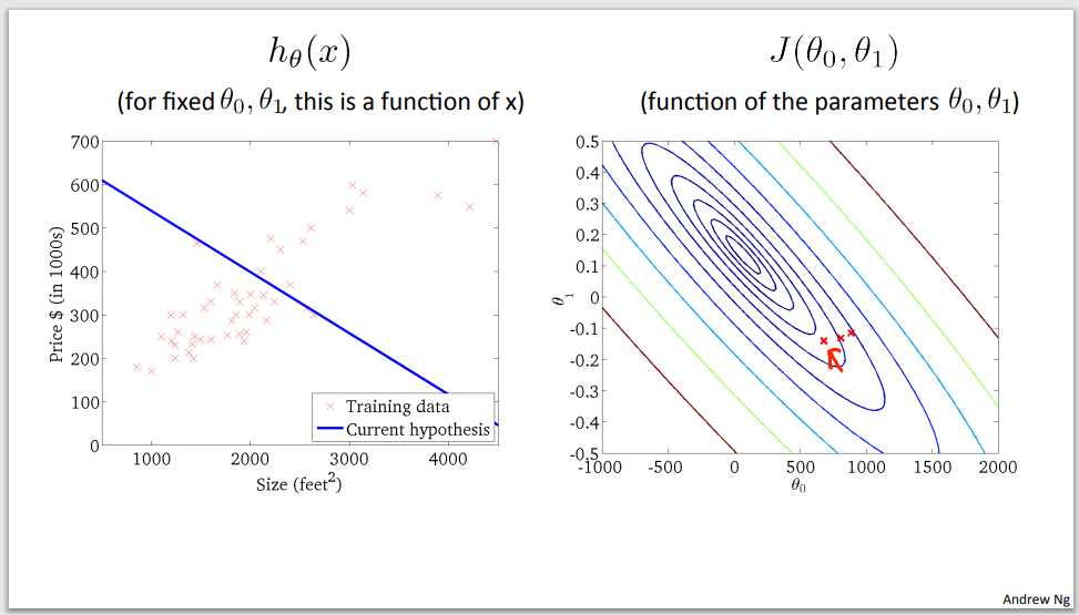
Step 2

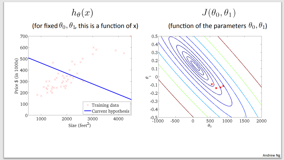
Step 3
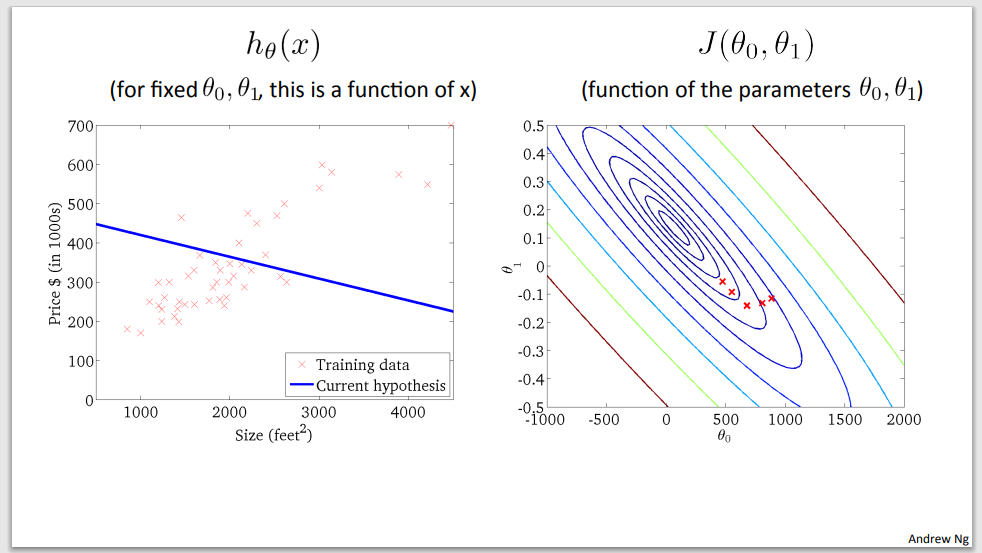
Step 4
Step 5
Step 6
Step 7
Step 8
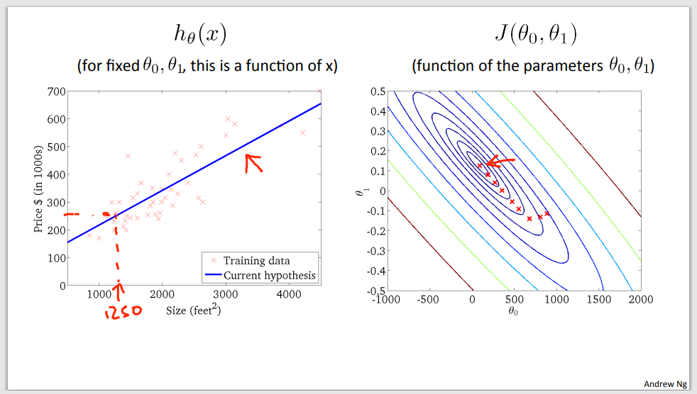
Step 9 – a good time to predict (global minimum was found)
Linear Algebra
- Matrices are two-dimensional arrays
\begin{bmatrix} a & b \\ c & d \\ e & f \end{bmatrix}
- Dimension: rows x columns
- 3×2 matrix =>
\R^{3x2}
- 3×2 matrix =>
- Entry:
A_{ij}->i^{th}row,j^{th}column
Ex. A_{12} = b
- Vector – matrix with one column and many rows
\begin{bmatrix} a \\ b \\ c \\ d \end{bmatrix}
- Dimension: n-dimensional vector
- 3-dimensional vector ->
\R^3
- 3-dimensional vector ->
Convention
- Uppercase letters – matrices (A, B, C, …)
- Lowercase letters – vectors (a, b, c, …)
Scalar
Single value – not a matrix or vector
Matrix addition
Add each corresponding element:
\begin{bmatrix} a & b \\ c & d \end{bmatrix} + \begin{bmatrix} w & x \\ y & z \end{bmatrix} = \begin{bmatrix} a + w & b + x \\ c + y & d + z \end{bmatrix}
Example:
\begin{bmatrix} 1 & 2 & 4 \\ 5 & 3 & 2 \end{bmatrix} + \begin{bmatrix} 1 & 3 & 4 \\ 1 & 1 & 3 \end{bmatrix} = \begin{bmatrix} 1 + 1 & 2 + 3 & 4 + 4 \\ 5 + 1 & 3 + 1 & 2 + 3 \end{bmatrix} = \begin{bmatrix} 2 & 5 & 8 \\ 6 & 4 & 1 \end{bmatrix}
Undefined for matrices with different dimension
Matrix subtracting
Subtract each corresponding element
\begin{bmatrix} a & b \\ c & d \end{bmatrix} - \begin{bmatrix} w & x \\ y & z \end{bmatrix} = \begin{bmatrix} a - w & b - x \\ c - y & d - z \end{bmatrix}
Example:
\begin{bmatrix} 1 & 2 & 4 \\ 5 & 3 & 2 \end{bmatrix} - \begin{bmatrix} 1 & 3 & 4 \\ 1 & 1 & 3 \end{bmatrix} = \begin{bmatrix} 1 - 1 & 2 - 3 & 4 - 4 \\ 5 - 1 & 3 - 1 & 2 - 3 \end{bmatrix} = \begin{bmatrix} 0 & -1 & 0 \\ 4 & 2 & -1 \end{bmatrix}
Undefined for matrices with different dimension
Scalar multiplication
Multiply each element by the scalar value
\begin{bmatrix} a & b \\ c & d \end{bmatrix} * x = \begin{bmatrix} a * x & b * x \\ c * x & d * x \end{bmatrix}
Example:
\begin{bmatrix} 1 & 2 & 4 \\ 5 & 3 & 2 \end{bmatrix} * 2 = \begin{bmatrix} 1 * 2 & 2 * 2 & 4 * 2 \\ 5 * 2 & 3 * 2 & 2 * 2 \end{bmatrix} = \begin{bmatrix} 2 & 4 & 8 \\ 10 & 6 & 4 \end{bmatrix}
Scalar division
Divide each element by the scalar value
\begin{bmatrix} a & b \\ c & d \end{bmatrix} / x = \begin{bmatrix} a / x & b / x \\ c / x & d / x \end{bmatrix}
Example:
\begin{bmatrix} 1 & 2 & 4 \\ 5 & 3 & 2 \end{bmatrix} / 2 = \begin{bmatrix} 1 / 2 & 2 / 2 & 4 / 2 \\ 5 / 2 & 3 / 2 & 2 / 2 \end{bmatrix} = \begin{bmatrix} 0.5 & 1 & 2 \\ 2.5 & 1.5 & 1 \end{bmatrix}
Matrix-Vector Multiplication
| A | x | X | = | Y |
|---|---|---|---|---|
\begin{bmatrix} & & & \\ & & & \end{bmatrix} |
x | \begin{bmatrix} & \\ & \\ & \end{bmatrix} |
= | \begin{bmatrix} & \\ & \end{bmatrix} |
mxn |
nx1 |
m-dimensional \ vector |
||
| (m rows, n columns) | (n-dimensional vector) |
To get y_i, multiply A’s i^{th} row with an element of vector x, and add them up:
\begin{bmatrix} a & b \\ c & d \\ e & f \end{bmatrix} * \begin{bmatrix} x \\ y \end{bmatrix} = \begin{bmatrix} a * x & b * y \\ c * x & d * y \\ e * x & f * y \end{bmatrix}
Example:
\begin{bmatrix} 1 & 2 & 3 \\ 4 & 5 & 6 \\ 7 & 8 & 9 \end{bmatrix} * \begin{bmatrix} 3 \\ 2 \\ 1 \end{bmatrix} = \begin{bmatrix} 1 * 3 & 2 * 2 & 3 * 1 \\ 4 * 3 & 5 * 2 & 6 * 1 \\ 7 * 3 & 8 * 2 & 9 * 1 \end{bmatrix} = \begin{bmatrix} 10 \\ 28 \\ 46 \end{bmatrix}
Matrix-Matrix Multiplication
| A | x | X | = | Y |
|---|---|---|---|---|
\begin{bmatrix} & & & \\ & & & \end{bmatrix} |
x | \begin{bmatrix} & & & \\ & & & \end{bmatrix} |
= | \begin{bmatrix} & & &\\ & & & \end{bmatrix} |
mxn matrix |
nxo matrix |
mxo matrix |
||
| (m rows, n columns) | (n rows, o columns) | (m rows, o columns) |
The i^{th} column of the matrix C is obtained by multiplying A with the ith column of B (for i = 1, 2,… o)
\begin{bmatrix} a & b \\ c & d \\ e & f\end{bmatrix} |
* |
\begin{bmatrix} w & x \\ y & z \end{bmatrix} |
= | \begin{bmatrix} a * w + b * y & a * x + b * z \\ c * w + d * y & c * x + d * z \\ e * w + f * y & e * x + f * z \end{bmatrix} |
|---|---|---|---|---|
\textcolor{blue}{3x2} |
\textcolor{blue}{2x2} |
\textcolor{blue}{3x2} |
Example:
\begin{bmatrix} 1 & 2 & 1 \\ 3 & 4 & 3 \\ 5 & 6 & 5 \end{bmatrix} * \begin{bmatrix} 1 & 2 \\ 3 & 2 \\ 1 & 3 \end{bmatrix} = \begin{bmatrix} 1 * 1 + 2 * 3 + 1 * 1 & 1 * 2 + 2 * 2 + 1 * 3 \\ 3 * 1 + 4 * 3 + 3 * 1 & 3 * 2 + 4 * 2 + 3 * 3 \\ 5 * 1 + 6 * 3 + 5 * 1 & 5 * 2 + 6 * 2 + 5 * 3 \end{bmatrix} = \begin{bmatrix} 8 & 9 \\ 18 & 23 \\ 28 & 37 \end{bmatrix}
Matrix Multiplication Properties
- Matrices are not commutative:
A * B != B * C - Matrices are associative:
(A * B) * C = A * (B * C)
Identity Matrix
Denoted I (or I_{nxn}) = simply – has 1’s in the diagonal (upper left to lower right diagonal) and 0’s elsewhere
Example:
\begin{bmatrix} 1 & 0 \\ 0 & 1 \end{bmatrix} \begin{bmatrix} 1 & 0 & 0 \\ 0 & 1 & 0 \\ 0 & 0 & 1 \end{bmatrix} \begin{bmatrix} 1 & 0 & 0 & 0 & ... \\ 0 & 1 & 0 & 0 & ... \\ 0 & 0 & 1 & 0 & ... \\ 0 & 0 & 0 & 1 & ... \\ ... & ... & ... & ... & 1 \\ \end{bmatrix}
For any matrix A
A * I = I * A = A
Matrix Inverse
If is an mxm matrix, and it has an inverse
A(A^{-1}) = A^{-1} * A = I
Matrices that don’t have an inverse are:
- Singular
- Degenerate
Matrix Transpose
Let A be on mxn matrix and let B = A^T
Then B is nxm matrix and
B_{ij} = A_{ji}
Example:
A = \begin{bmatrix} 1 & 2 & 0 \\ 3 & 5 & 9 \end{bmatrix} B = A^T \begin{bmatrix} 1 & 3 \\ 2 & 5 \\ 0 & 9 \end{bmatrix}
The first row of A becomes first columns of A^T