Change prompt
from octave:1>` to `>>
octave:1> PS1('>> ');
>>
Help command
>> help help
'help' is a function from the file C:\Octave\OCTAVE~1.0\mingw64\share\octave\5.2.0\m\help\help.m

 -- help NAME
 -- help --list
 -- help .
 -- help
     Display the help text for NAME.

     For example, the command 'help help' prints a short message
     describing the 'help' command.

     Given the single argument '--list', list all operators, keywords,
     built-in functions, and loadable functions available in the current
     session of Octave.

     Given the single argument '.', list all operators available in the
     current session of Octave.

     If invoked without any arguments, 'help' displays instructions on
     how to access help from the command line.

     The help command can provide information about most operators, but
     NAME must be enclosed by single or double quotes to prevent the
     Octave interpreter from acting on NAME.  For example, 'help "+"'
     displays help on the addition operator.

     See also: doc, lookfor, which, info.

Additional help for built-in functions and operators is
available in the online version of the manual.  Use the command
'doc <topic>' to search the manual index.

Help and information about Octave is also available on the WWW
at https://www.octave.org and via the help@octave.org
mailing list.
Basic Operations
Math Operations
Addition
>> 5+6
ans = 11
Subtraction
>> 3-2
ans = 1
Multiplication
>> 5*8
ans = 40
Division
>> 1/2
ans = 0.50000
Exponent
>> 2^6
ans = 64
Logic operations
Equality
>> 1 == 2
ans = 0
Inequality
>> 1 ~= 2
ans = 1
Logical AND
>> 1 && 0
ans = 0
Logical OR
>> 1 || 0
ans = 1
Logical XOR
>> xor(1,0)
ans = 1
Variables
Assignments
numbers
>> a =3;
>> a
a = 3
strings
>> b = 'hi';
>> b
b = 'hi'
calculations
>> c = (3>=1);
>> c
c = 1
$\pi$
>> a = pi;
>> a
>> a = 3.1416
Displaying Variables
numbers
>> a = pi;
>> disp(a)
3.1416
strings
>> a = pi;
>> disp(sprintf('2 decimals: %0.2f', a));
2 decimals: 3.14
>> disp(sprintf('6 decimals: %0.6f', a));
6 decimals: 3.141593
format
>> a = pi;
>> format long
>> a
a = 3.14159165358979
>> format short
>> a
a = 3.1416
Matrices
3×2 matrix
>> A = [1 2; 3 4; 5 6]
A =
    1   2
    3   4
    5   6
or
>> A = [1 2;
> 3 4;
> 5 6]
A =
    1   2
    3   4
    5   6
1×3 Matrix
>> V = [1 2 3 ]
V =
    1   2   3
3×1 Vector
>> V = [1; 2; 3;]
V =
    1
    2
    3
Creating vector from 1 to 2 increasing next element by 0.1
>> V = 1:0.1:2
V =
    1.0000    1.1000    1.2000    1.3000    1.4000    1.5000    1.6000    1.7000    1.8000    1.9000    2.0000
Creating vector from 1 to 6 increasing next element by 1
>> V = 1:6
V =
    1   2   3   4   5   6
Matrix 2×3 with all values eqauls 1
>> ones(2,3)
ans =
    1   1   1
    1   1   1
Matrix 2×3 with all values eqauls 2
>> C = 2*ones(2,3)
C =
    2   2   2
    2   2   2
Row vector with 1
>> w = ones(1,3)
w =
    1   1   1
Row vector with 0
>> w = zeros(1,3)
w =
    0   0   0
Random matrix (numbers between 0 and 1)
>> rand(1,3)
ans =
   0.32784   0.49321   0.17449
>> rand(3,3)
ans =
   0.60369   0.15891   0.75957
   0.47148   0.11786   0.86370
   0.46272   0.51486   0.71124
Gaussian random variables
>> randn(1,3)
ans =
  -0.67605  -0.54028   0.42763
More complicated
>> w = -6 + sqrt(10)*randn(1,100)
w =
 Columns 1 through 8:
   -4.5865653   -8.8356479   -8.1333614   -2.3439273   -7.3621630   -9.0450181   -2.1489934   -4.2785162
 Columns 9 through 16:
  -10.7109066   -7.5124041   -6.6674847  -14.4887638   -0.4808289   -2.1354753   -7.8977581   -8.9314986
 Columns 17 through 24:
   -8.9893458   -1.5510572  -10.3796268  -10.2004881   -1.9258233  -10.7401729   -1.4114864  -11.9918739
 Columns 25 through 32:
   -1.4288672   -9.1350859   -4.0339111   -7.1057222   -5.5066692   -5.3943613   -9.9372854  -12.3273985
 Columns 33 through 40:
   -9.1448272   -3.5632437   -9.8825123   -3.6862963   -0.9314631   -7.1585643   -7.5249914   -6.7338681
 Columns 41 through 48:
   -4.0692604   -3.1736484   -7.1340077   -5.6141781   -7.1375287  -10.1554003   -7.3884758   -8.2993959
 Columns 49 through 56:
   -7.9971092   -3.7486347   -4.9565946  -10.1077235   -3.7186839   -7.6239998   -9.3567788   -7.0285528
 Columns 57 through 64:
   -5.7498064   -5.1235503    2.6385315   -7.0795552   -5.1845500   -2.7447164   -7.7785950    0.8816560
 Columns 65 through 72:
   -6.5335031    0.0066014   -3.9586199   -2.1445580   -3.4484948  -12.8979017   -1.5233025   -4.4102424
 Columns 73 through 80:
    0.9831482   -4.7574813   -2.7595514  -11.2178766   -5.3229671   -1.8543523   -3.7577500   -3.8678680
 Columns 81 through 88:
   -3.8637871   -7.2037168  -11.7877396   -7.1542280   -7.5999564    0.2206099   -6.7140798   -1.3302397
 Columns 89 through 96:
   -3.6058713   -5.5103303   -5.8951690   -1.6396029   -8.2389941   -4.5821969   -4.4162341   -6.9883700
 Columns 97 through 100:
   -3.4562746   -3.8389149   -0.8080181   -4.6449049
   ```

#### Histagram
```r
>> hist(w)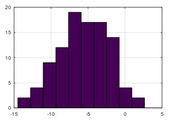
>> hist(w,50)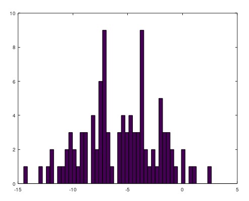
>> eye(4)
ans =
Diagonal Matrix
   1   0   0   0
   0   1   0   0
   0   0   1   0
   0   0   0   1
Moving Data Around
Matrices size
>> A = [1 2; 3 4; 5 6]
A =
   1   2
   3   4
   5   6

>> size(A)
ans =
   3   2
Get dimensions (rows) of Matrix
>> size(A,1)
ans =  3
Get number of columns
>> size(A,2)
ans =  2
Length of Vector
V =
   4   3   1   5
>> length(V)
ans =  4
It can be applied as well to Matrices, but then the result will be only for the longest dimension
>> length(A)
ans =  3
Loading data
Show the current directory
>> pwd
ans = C:\Users\Gosia
Changing directory
>> cd 'D:\Projects'
>> pwd
ans = D:\Projects
Load data
>> load data.txtdisplay data from the file
>> data
data =
    6.11010   17.59200
    5.52770    9.13020
    8.51860   13.66200
    7.00320   11.85400
    5.85980    6.82330
    8.38290   11.88600
    7.47640    4.34830
    8.57810   12.00000
    6.48620    6.59870
    5.05460    3.81660
    5.71070    3.25220
   14.16400   15.50500
    5.73400    3.15510
    8.40840    7.22580
    5.64070    0.71618
    5.37940    3.51290
    6.36540    5.30480
    5.13010    0.56077
    6.42960    3.65180
    7.07080    5.38930
    6.18910    3.13860
check the size of data (file)
>> size(data)
ans =
   97    2
check variables that Octave has in memory
>> who
Variables in the current scope:
A     V     a     ans   b     c     data  w
check variables with details that Octave has in memory
>> whos
Variables in the current scope:

   Attr Name        Size                     Bytes  Class
   ==== ====        ====                     =====  =====
        A           3x2                         48  double
        V           1x4                         32  double
        a           1x1                          8  double
        ans         1x2                         16  double
        b           1x2                          2  char
        c           1x1                          1  logical
        data       97x2                       1552  double
        w           1x100                      800  double

Total is 310 elements using 2459 bytes
assign only selected data from one variable to another
>> m = data(1:10)
m =

   6.1101   5.5277   8.5186   7.0032   5.8598   8.3829   7.4764   8.5781   6.4862   5.0546

>> whos
Variables in the current scope:

   Attr Name        Size                     Bytes  Class
   ==== ====        ====                     =====  =====
        A           3x2                         48  double
        V           1x4                         32  double
        a           1x1                          8  double
        ans         1x2                         16  double
        b           1x2                          2  char
        c           1x1                          1  logical
        data       97x2                       1552  double
        m           1x10                        80  double
        w           1x100                      800  double

Total is 320 elements using 2539 bytes
save a variable to a file (in binary format)
>> save hello.mat m;
>> ls
 Volume in drive D is Data
 Volume Serial Number is 9C15-10B4

 Directory of D:\machine-learning-ex\test

[.]         [..]        data.txt    hello.mat
               2 File(s)          1,691 bytes
               2 Dir(s)  88,129,142,784 bytes free
save a variable to a file (in ascii format)
>> save hello.txt m -asciihello.txt
6.11010000e+00 5.52770000e+00 8.51860000e+00 7.00320000e+00 5.85980000e+00 8.38290000e+00 7.47640000e+00 8.57810000e+00 6.48620000e+00 5.05460000e+00clear selected variable
>> clear data
>> whos
Variables in the current scope:

   Attr Name        Size                     Bytes  Class
   ==== ====        ====                     =====  =====
        A           3x2                         48  double
        V           1x4                         32  double
        a           1x1                          8  double
        ans         1x2                         16  double
        b           1x2                          2  char
        c           1x1                          1  logical
        w           1x100                      800  double

Total is 116 elements using 907 bytes
clear all variables
>> clear
>> whos
>>
loading saved variable
>> load hello.mat
>> whos
Variables in the current scope:

   Attr Name        Size                     Bytes  Class
   ==== ====        ====                     =====  =====
        m           1x10                        80  double

Total is 10 elements using 80 bytes
Get specific element from the variable (example: 3rd column and 2nd row)
>> A=[1 2; 3 4; 5 6]
A =

   1   2
   3   4
   5   6

>> A(3,2)
ans =  6
Get everything in a second row
>> A(2,:)
ans =
   3   4
Get everything in a second column
>> A(:,2)
ans =

   2
   4
   6
Get all elements from specific columns
>> A([1 3],:)
ans =

   1   2
   5   6

>> A([2 3],:)
ans =

   3   4
   5   6

>> A([1 2 3],:)
ans =

   1   2
   3   4
   5   6
Change data in matrix
>> A
A =

   1   2
   3   4
   5   6

>> A(:,2) = [10;11;12]
A =

    1   10
    3   11
    5   12
Add (append) another column vector data to the right
>> A = [A, [100; 101; 102]];
>> A
A =

     1    10   100
     3    11   101
     5    12   102
Put all element of matrix into single column vector
>> A(:)
ans =

     1
     3
     5
    10
    11
    12
   100
   101
   102
Combine two matrices
>> A = [1 2; 3 4; 5 6];
>> B = [11 12; 13 14; 15 16];
>> C = [A B]
C =

    1    2   11   12
    3    4   13   14
    5    6   15   16
or
>> A = [1 2; 3 4; 5 6];
>> B = [11 12; 13 14; 15 16];
>> C = [A; B]
C =

    1    2
    3    4
    5    6
   11   12
   13   14
   15   16
Computing on Data
Multiply
>> A = [1 2; 3 4; 5 6];
>> C = [1 1; 2 2];
>> A*C
ans =

    5    5
   11   11
   17   17
Element-wise multiplication
>> A = [1 2; 3 4; 5 6];
>> B = [11 12; 13 14; 15 16];
>> A .*B
ans =

   11   24
   39   56
   75   96
Element-wise squaring
>> A = [1 2; 3 4; 5 6];
>> A .^ 2
ans =

    1    4
    9   16
   25   36
Element-wise Reciprocal
>> V = [1; 2; 3];
>> 1 ./ V
ans =

   1.00000
   0.50000
   0.33333
Element-wise inverse of A (matrix)
>> A = [1 2; 3 4; 5 6];
>> 1 ./A
ans =

   1.00000   0.50000
   0.33333   0.25000
   0.20000   0.16667
Element-wise logarithm
>> V = [1; 2; 3];
>> log(V)
ans =

   0.00000
   0.69315
   1.09861
Exponentiation
>> V = [1; 2; 3];
>> exp(V)
ans =

    2.7183
    7.3891
   20.0855
Element-wise absolute value
>> V = [1; 2; 3];
>> abs(V)
ans =

   1
   2
   3

>> abs([-1; -3; -10])
ans =

    1
    3
   10
negative
>> V = [1; 2; 3];
>> -V
ans =

  -1
  -2
  -3
or
>> V = [1; 2; 3];
>> -1*V
ans =

  -1
  -2
  -3
Increment all values by one
>> V = [1; 2; 3];
>> V + ones(length(V),1)
ans =

   2
   3
   4
or
>> V = [1; 2; 3];
>> V + 1
ans =

   2
   3
   4
Matrix transport
>> A = [1 2; 3 4; 5 6];
>> A'
ans =

   1   3   5
   2   4   6
Max value
>> a = [1 15 2 0.5];
>> max(a)
ans =  15
Max value and index of this max value
>> val = max(a)
val =  15
>> [val, ind] = max(a)
val =  15
ind =  2
Column-wise maximum (on matrices)
>> A = [1 2; 3 4; 5 6];
>> max(A)
ans =

   5   6
or
>> A = [1 2; 3 4; 5 6];
>> max(A,[],1)
ans =

   5   6
Row-wise maximum (on matrices)
>> A = [1 2; 3 4; 5 6];
>> max(A,[],2)
ans =

   2
   4
   6
The max element in whole matrix
>> A = [1 2; 3 4; 5 6];
>> max(max(A))
ans =  6
or turn into vector
>> A = [1 2; 3 4; 5 6];
>> max(A(:))
ans =  6
Element-wise comparison (showing true/false)
>> a = [1 15 2 0.5];
>> a < 3
ans =

  1  0  1  1
Element-wise comparison (showing with element)
>> a = [1 15 2 0.5];
>> find(a < 3)
ans =

   1   3   4
Magic (N-by-N magic square)
>> A = magic(3)
A =

   8   1   6
   3   5   7
   4   9   2
>> A = magic(9)
A =
47 58 69 80 1 12 23 34 45
57 68 79 9 11 22 33 44 46
67 78 8 10 21 32 43 54 56
77 7 18 20 31 42 53 55 66
6 17 19 30 41 52 63 65 76
16 27 29 40 51 62 64 75 5
26 28 39 50 61 72 74 4 15
36 38 49 60 71 73 3 14 25
37 48 59 70 81 2 13 24 35sum columns
>> sum(A,1)
ans =

   369   369   369   369   369   369   369   369   369
sum rows
>> sum(A,2)
ans =

   369
   369
   369
   369
   369
   369
   369
   369
   369
sum diagonal
>> eye(9)
ans =

Diagonal Matrix

   1   0   0   0   0   0   0   0   0
   0   1   0   0   0   0   0   0   0
   0   0   1   0   0   0   0   0   0
   0   0   0   1   0   0   0   0   0
   0   0   0   0   1   0   0   0   0
   0   0   0   0   0   1   0   0   0
   0   0   0   0   0   0   1   0   0
   0   0   0   0   0   0   0   1   0
   0   0   0   0   0   0   0   0   1

>> A .* eye(9)
ans =

   47    0    0    0    0    0    0    0    0
    0   68    0    0    0    0    0    0    0
    0    0    8    0    0    0    0    0    0
    0    0    0   20    0    0    0    0    0
    0    0    0    0   41    0    0    0    0
    0    0    0    0    0   62    0    0    0
    0    0    0    0    0    0   74    0    0
    0    0    0    0    0    0    0   14    0
    0    0    0    0    0    0    0    0   35

>> sum(sum(A.*eye(9)))
ans =  369

>> flipud(eye(9))
ans =

Permutation Matrix

   0   0   0   0   0   0   0   0   1
   0   0   0   0   0   0   0   1   0
   0   0   0   0   0   0   1   0   0
   0   0   0   0   0   1   0   0   0
   0   0   0   0   1   0   0   0   0
   0   0   0   1   0   0   0   0   0
   0   0   1   0   0   0   0   0   0
   0   1   0   0   0   0   0   0   0
   1   0   0   0   0   0   0   0   0

>> sum(sum(A.*flipud(eye(9))))
ans =  369
finding by row and column
>> A = magic(3);
>> [r,c] = find(A >= 7)
r =

   1
   3
   2

c =

   1
   2
   3

>> [row,column] = find(A >= 7)
row =

   1
   3
   2

column =

   1
   2
   3
Pseudo-inverse
>> A = magic(3)
A =

   8   1   6
   3   5   7
   4   9   2

>> pinv(A)
ans =

   0.147222  -0.144444   0.063889
  -0.061111   0.022222   0.105556
  -0.019444   0.188889  -0.102778
Add all elements
>> a = [1 15 2 0.5];
>> sum(a)
ans =  18.500
Multiply all elements
>> a = [1 15 2 0.5];
>> prod(a)
ans =  15
Rounds down elements ( Return the largest integer not greater than X)
>> a = [1 15 2 0.5];
>> floor(a)
ans =

    1   15    2    0
Rounds up elements ( Return the smallest integer not less than X)
>> a = [1 15 2 0.5];
>> ceil(a)
ans =

    1   15    2    1
Plotting Data
Sample generated data for the plot (numbers from 0 to up 0.98) and sin function
>> t=[0:0.01:0.98];
>> y1 = sin(2*pi*4*t);
Generating plot, where horizontal axis = t and verical axis = y1:
>> plot(t,y1);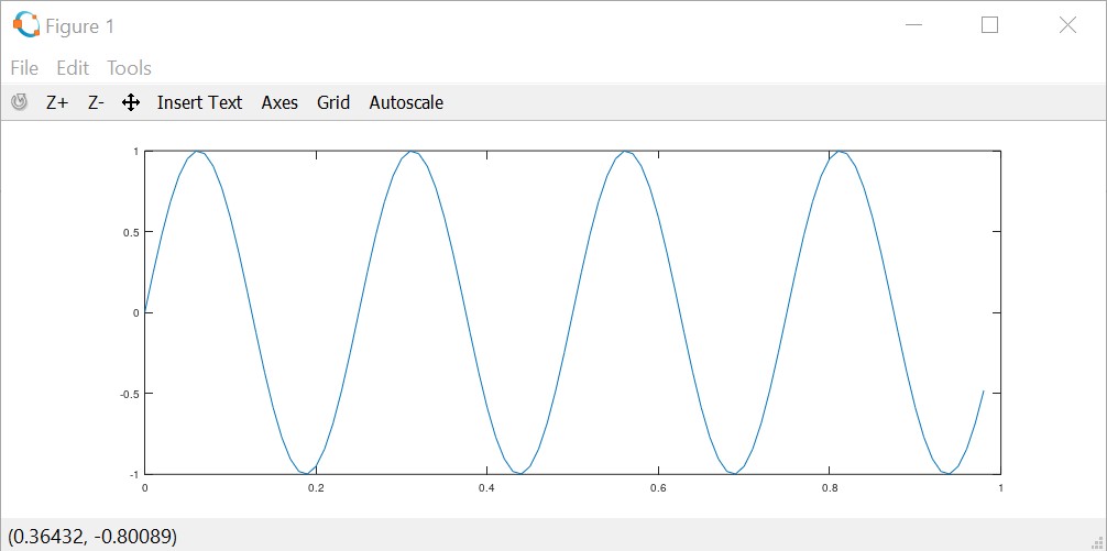
When run once again the plot with different argument, it will be replaced with new plot:
>> y2 = cos(2*pi*4*t);
>> plot(t,y2);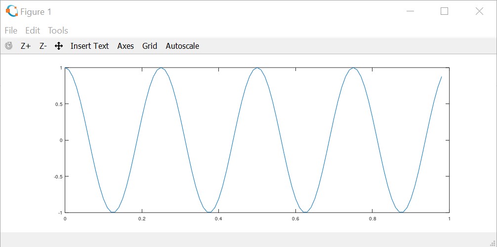
To have both (or more) plots on one designer it's needed to use the ```hold on;``` function:
>> plot(t,y1);
>> hold on;
>> plot(t,y2);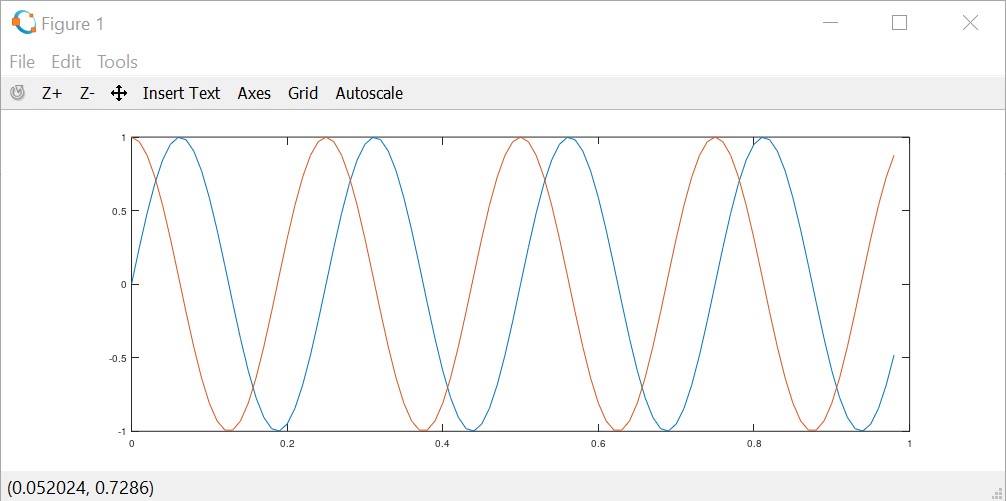
Adding labels, legend and title
>> xlabel('time');
>> ylabel('value');
>> legend('sin','cos');
>> title('my plot');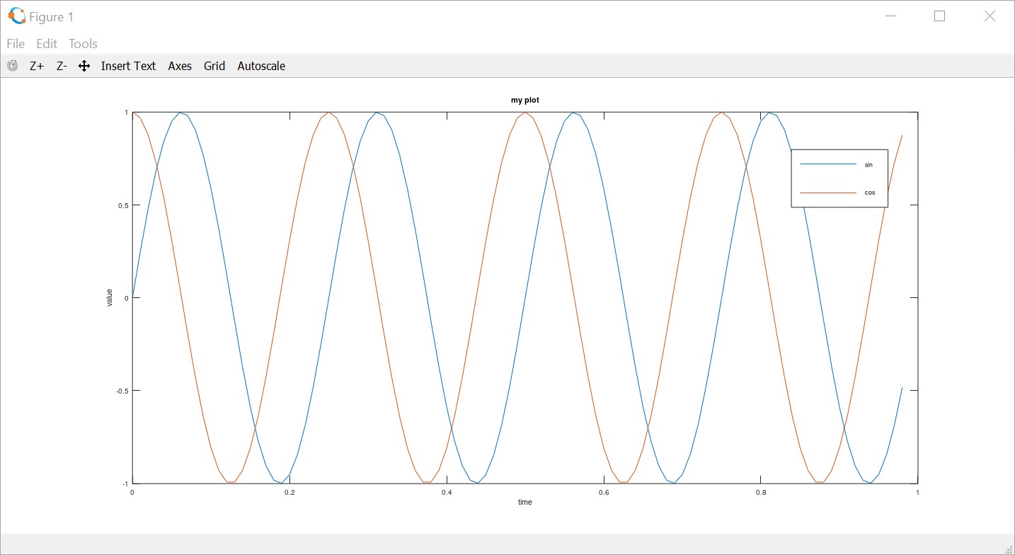
Saving the figure
>> cd D:\; print -dpng 'myPlot.png'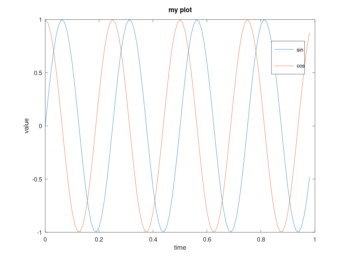
To close figure
>> close;To open two figures in seperate windows:
>> figure(1); plot(t,y1);
>> figure(2); plot(t,y2);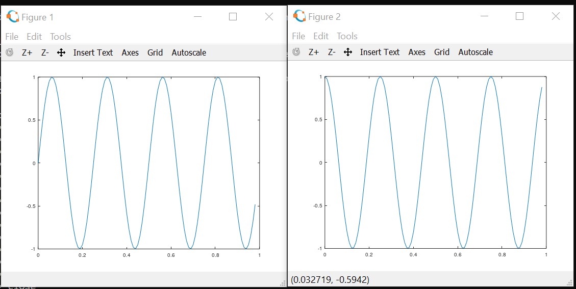
Dividing plot by 1x2 grid and access first element and next second element
>> subplot(1,2,1);
>> plot(t,y1);
Clear figure
>> clf;Visualize matrix
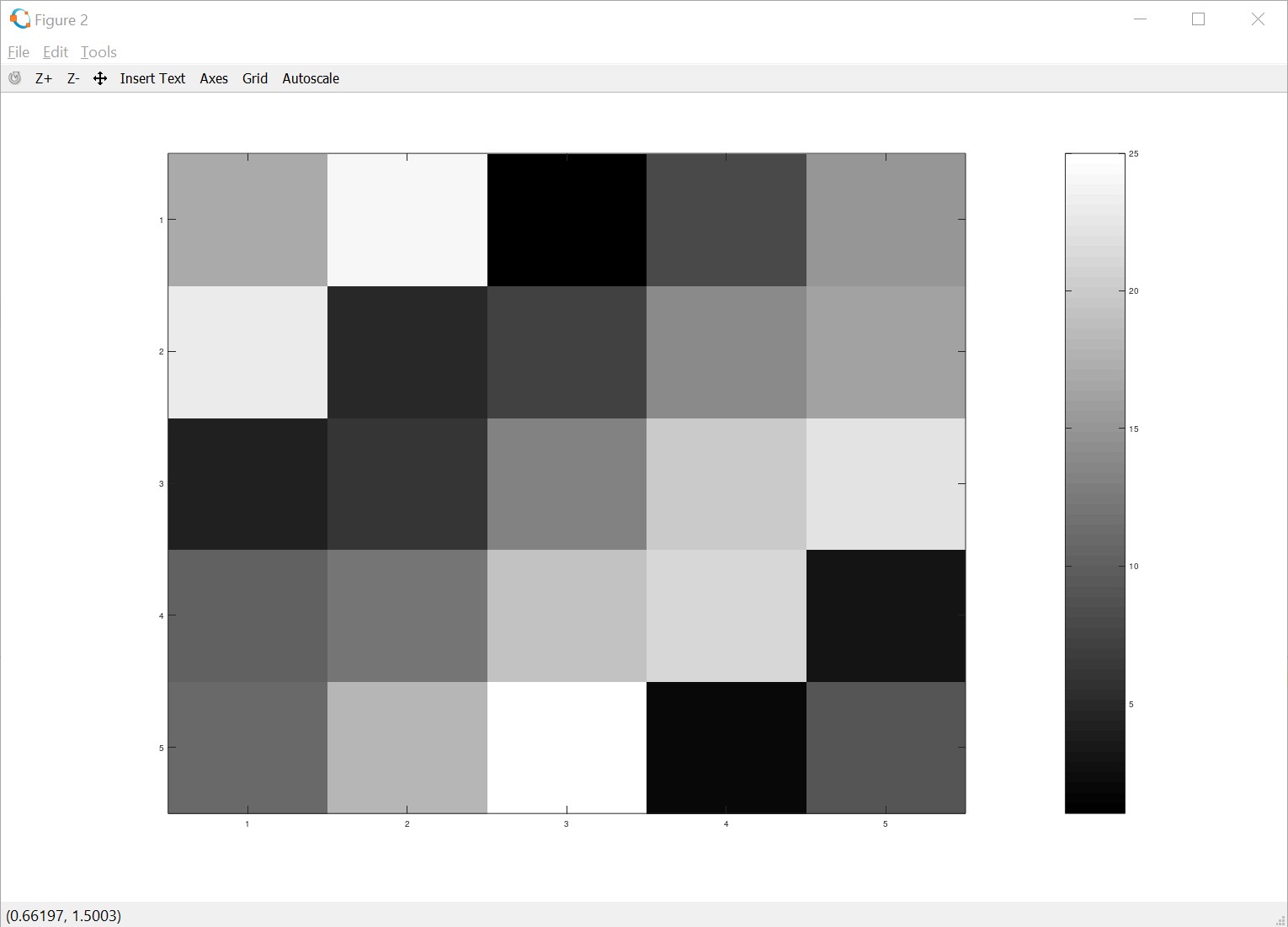
>> A = magic(5)
A =

   17   24    1    8   15
   23    5    7   14   16
    4    6   13   20   22
   10   12   19   21    3
   11   18   25    2    9

>> imagesc(A)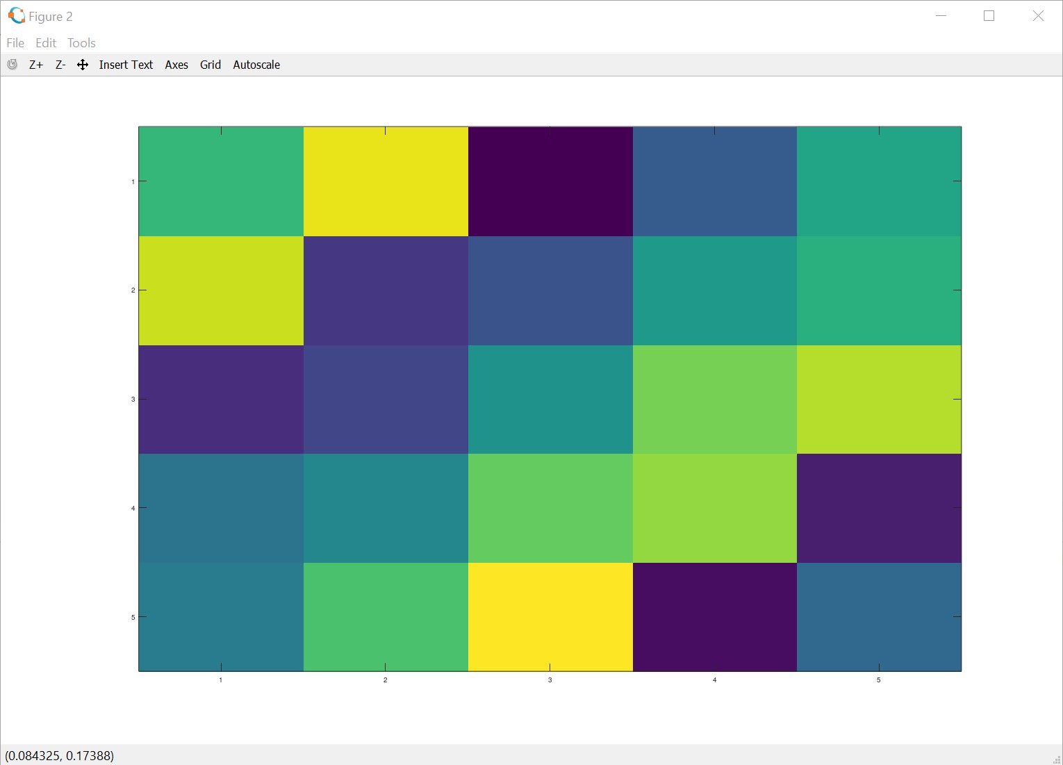
To show with grey colour with colour bar
>> imagesc(A), colorbar, colormap gray;