My notes from the Machine Learning Course provided by Andrew Ng on Coursera

Logistic Regression

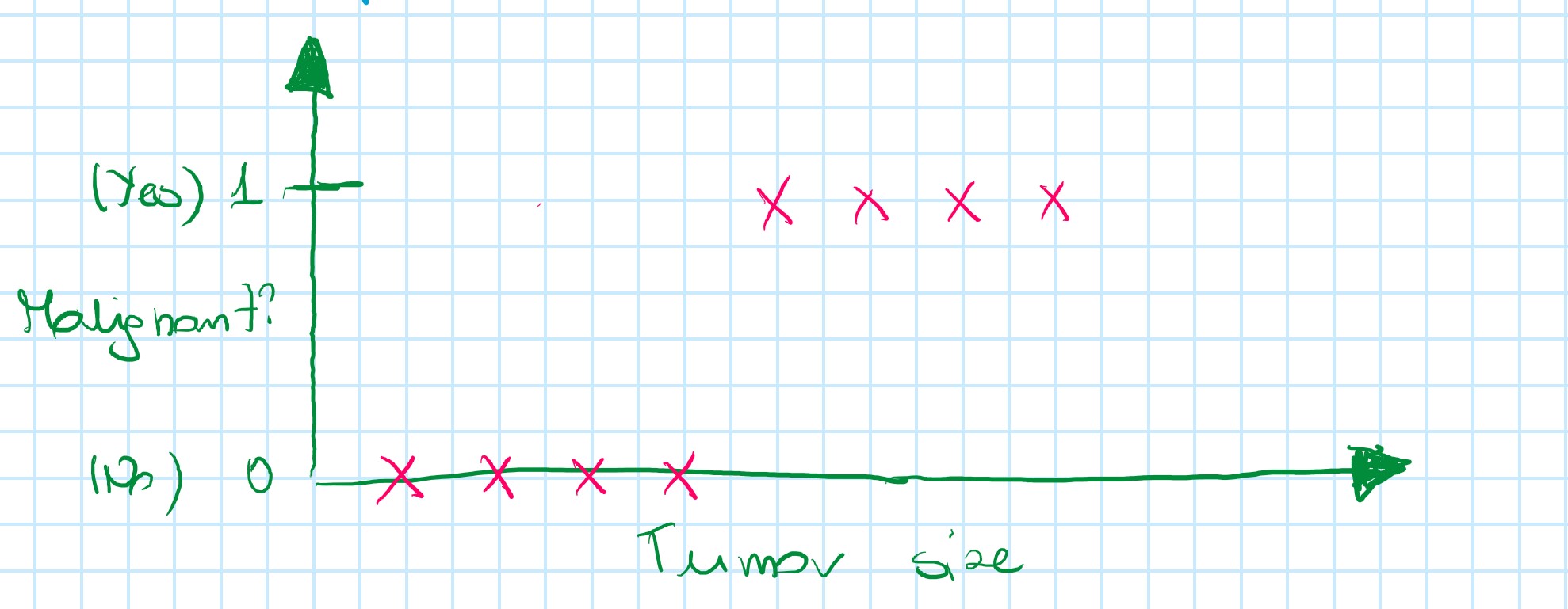
Example of classification problem:

Email: Spam/Not spam?
Online transaction: Fraudulent (Yes/No)?
Tumour: Malignant/Benign?

$y \in \{0,1\}$ where
$0$ – "Negative class"
$1$ – "Positive class"

Multiclass classification problem $y \in \{0,1,2,3,...\}$

How to develop a classification algorithm?

Example of a training set for classification task:

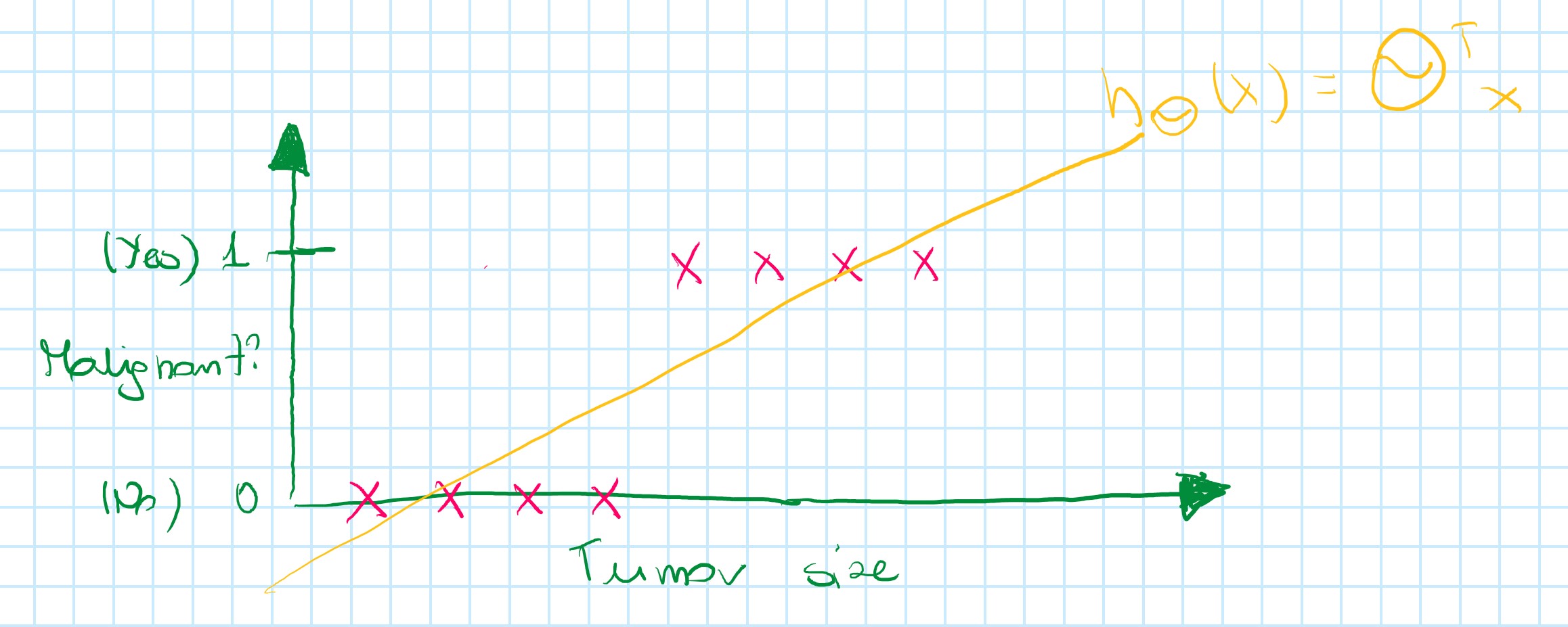
For this data set applying linear regression algorithm:
$h_{\theta}(x)=\theta^Tx$
and it could finish like below:

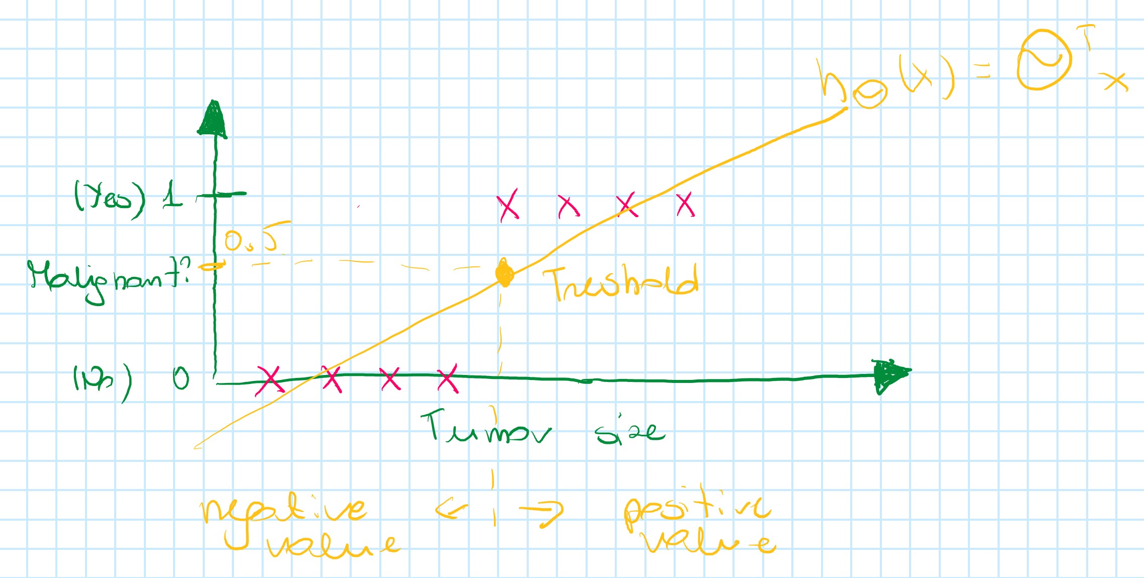
For prediction, it could be useful to try to do the threshold:

Threshold classifier output $h_{\theta}(x)$ at $0.5$ : (vertical axis value)

If $h_{\theta}(x) \geqslant 0.5$ , predict " $y=1$ "
If $h_{\theta}(x) < 0.5$ , predict " $y=0$ "

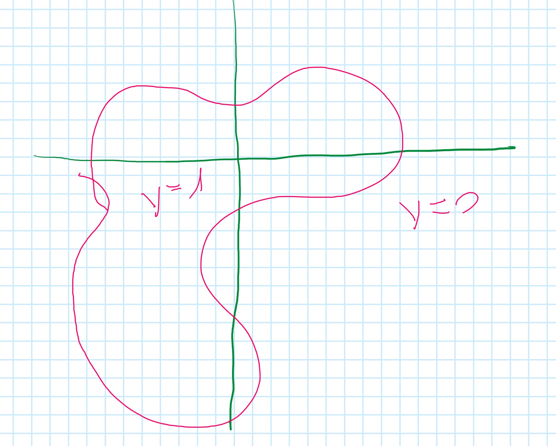
What happens if a problem will change a bit?

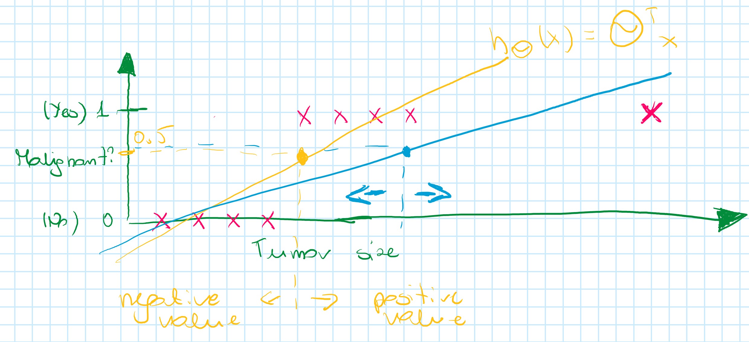
By adding one positive example cause linear regression to change, it's a straight line to fit the new data. It causes (in this example) a worse hypothesis.

Conclusion: Applying linear regression to classification problem often isn't a good idea

Funny bit of using linear regression on classification problem:
Classification: $y=0$ or $y=1$ but $h_{\theta}(x)$ can be $>1$ or $<0$
So even when if we know that label should be $0$ or $1$ , the linear regression could back with output values much larger than $1$ or much smaller than $0$ .

Logistic Regression: $0 \leqslant h_{\theta}(x) \leqslant 1$ - it's classification algorithm

Hypothesis Representation

Logistic Regression Model

Want $0 \leqslant h_{\theta}(x) \leqslant 1$

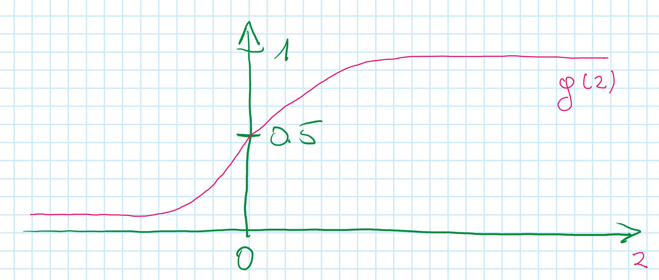
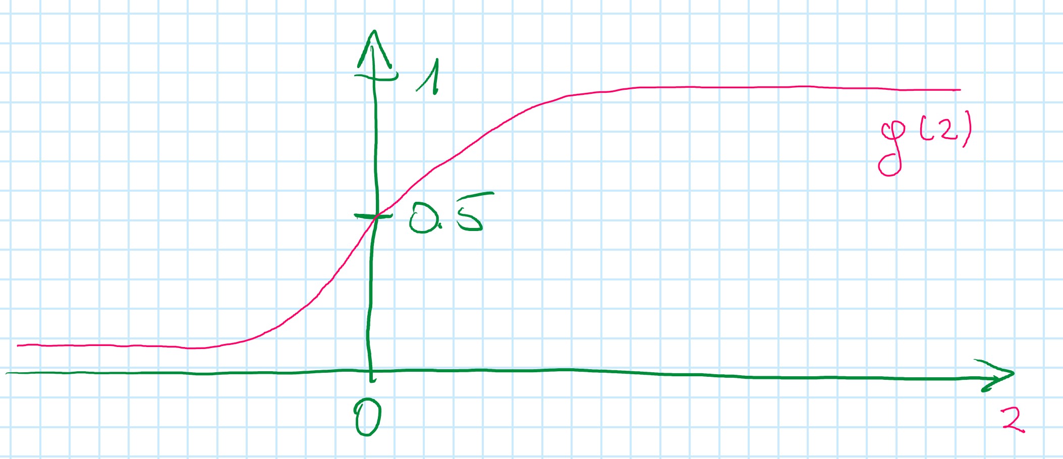
$h_{\theta}(x) = g(\theta^Tx)$

$g(z) = {1 \over {1 + e^{-z}}}$ (two different names for the same function: sigmoid function and logistic function )

$\begin{rcases} h_{\theta}(x) = g(\theta^Tx) \\ g(z) = {1 \over {1 + e^{-z}}} \end{rcases}⇒h_{\theta}(x)={1 \over {1 + e^{-\theta^Tx}}}$

$z$ - real number

Sigmoid function

Parameters: $\theta$

Interpretation of Hypothesis Output

$h_{\theta}(x)$ - estimated probability that $y=1$ on input $x$

Example:
$\text{if } x = \begin{bmatrix} x_0 \\ x_1 \end{bmatrix} = \begin{bmatrix} 1 \\ \text{tumor size} \end{bmatrix}$

$h_{\theta}(x) = 0.7$
Tell patient that 7-% chance of tumour being malignant

$h_{\theta}(x) = P(y=1|x;\theta)$ - probability that $y=1$ , give $x$ , parameterized by $\theta$

Because this is a classification problem, then $y$ can get only two values: $0$ or $1$

$P(y=0|x;\theta) + P(y=1|x;\theta) = 1$

$P(y=0|x;\theta) = 1 - P(y=1|x;\theta)$

Decision Boundary

Logistic Regression:

$h_{\theta}(x) = g(\theta^Tx)$

$g(z) = {1 \over {1 + e^{-z}}}$

Predict $"y=1"$ if $h_{\theta}(x) \geqslant 0.5$

Predict $"y=0"$ if $h_{\theta}(x) < 0.5$

$g(z) \geqslant 0.5$ when $z \geqslant 0$

$h_{\theta}(x) = g(\theta^Tx) \geqslant 0.5$ where $\theta^Tx \geqslant 0$

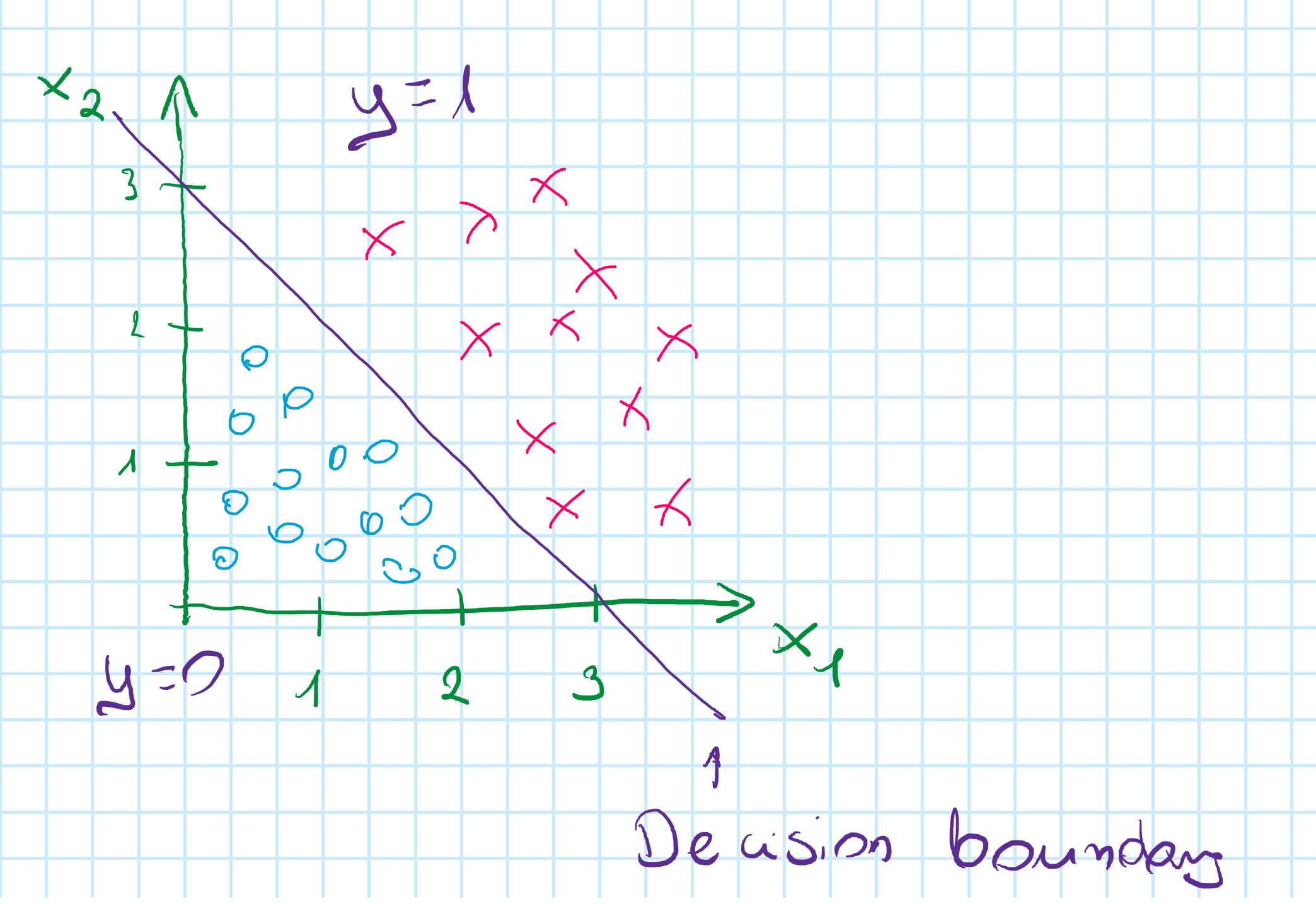
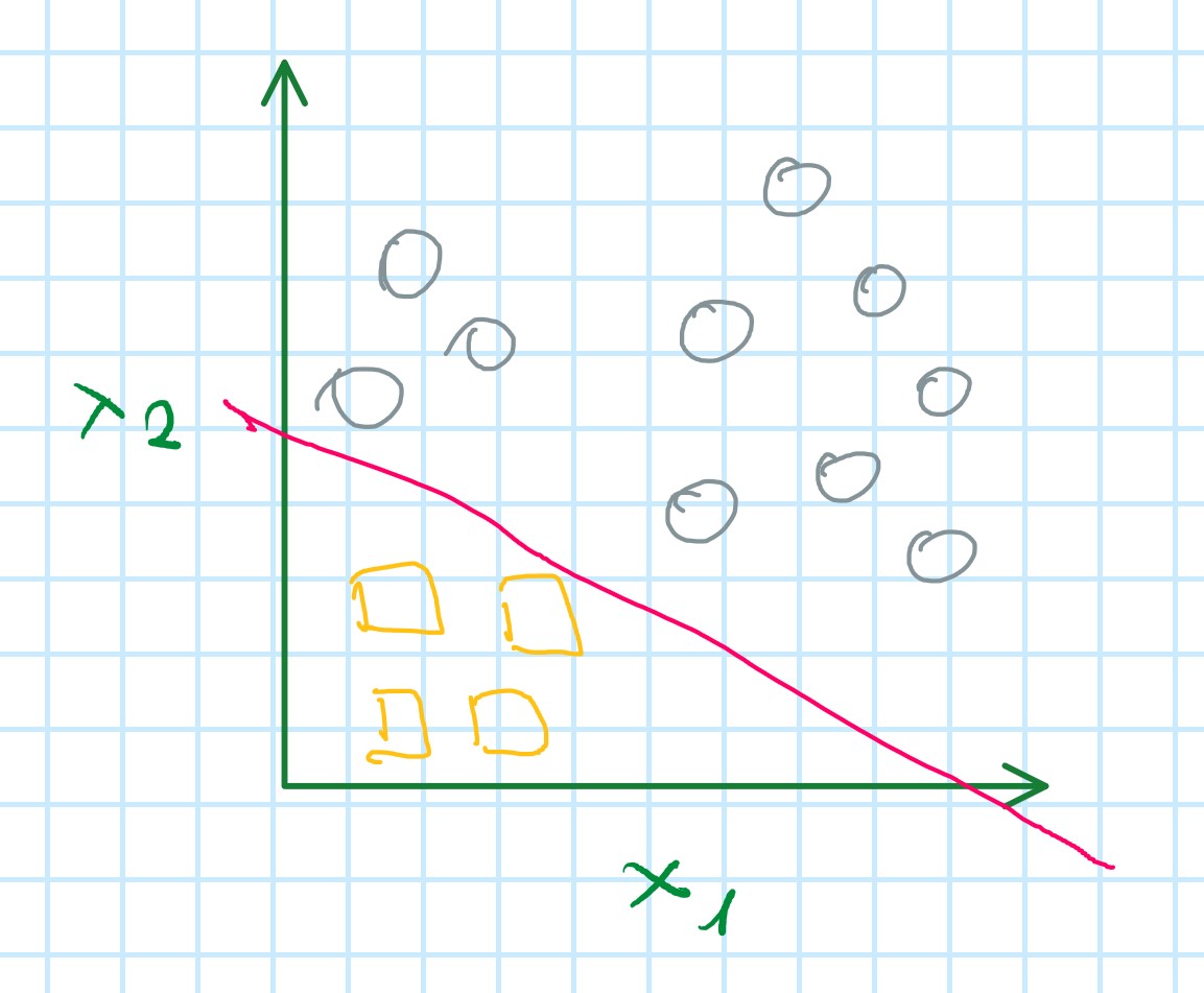
Training set

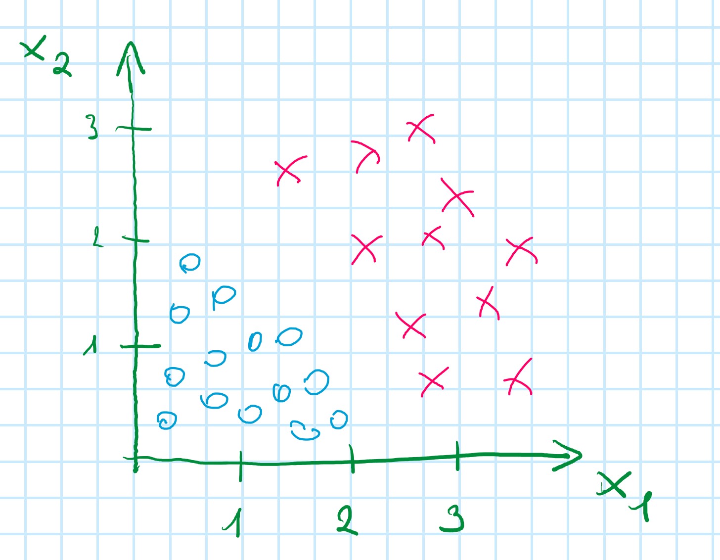
$h(_{\theta}(x) = q(\theta_0 + \theta_1x_1 + \theta_2x_2)$

Based on the plot: $h(_{\theta}(x) = q(-3 + 1x_1 + 1x_2)$

so: $\theta = \begin{bmatrix} -3 \\ 1 \\ 1 \end{bmatrix}$

Predict: $"y=1"$ if $-3 + x_1 + x_2 \geqslant 0$

$-3 + x_1 + x_2 \geqslant 0$

$x_1 + x_2 \geqslant 3$ - will create a straight line

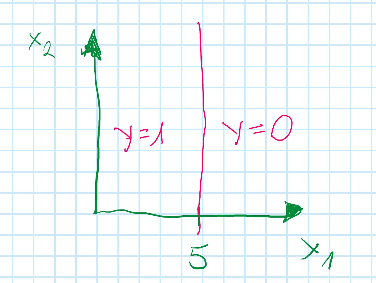
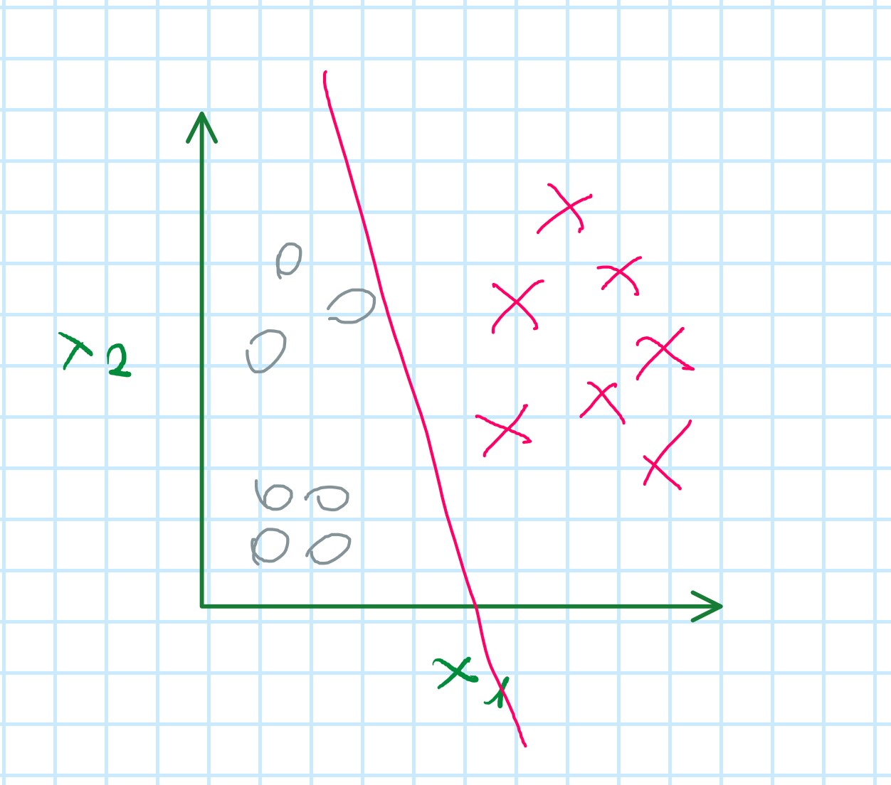
Exercise:

$\theta_0=5; \theta_1=-1; \theta_2=0;$

$h_{\theta}(x) = g(5-x_1)$

so: $x_1 \geqslant 5$

Non-linear decision boundaries

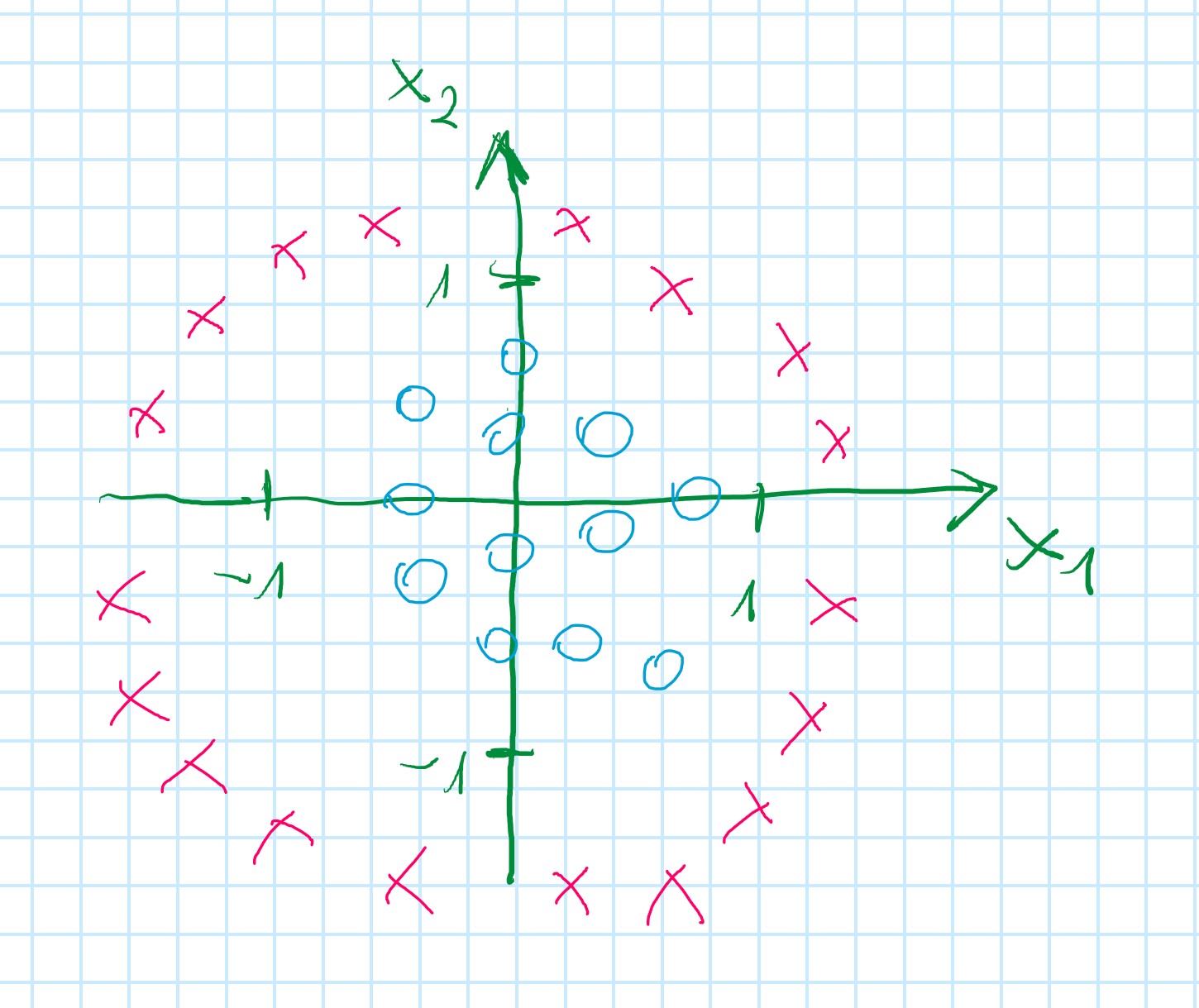
$h_{\theta}(x) = g(\theta_0 +\theta_2x_2 + \theta_3x_1^2 + \theta_4x_2^2)$

$\theta = \begin{bmatrix} -1 \\ 0 \\ 0 \\ 1 \\ 1 \end{bmatrix}$

Predict $"y=1"$ if $-1 + x_1^2 + x_2^2 \geqslant 0$

$x_1^2 + x_2^2 = 1$

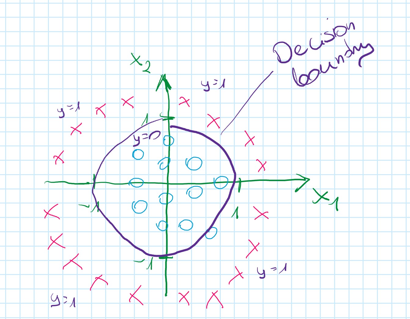
More complex decision boundaries

$h_{\theta}(x) = g(\theta_0 +\theta_2x_2 + \theta_3x_1^2 + \theta_4x_2^2 + \theta_5x_1^2x_2^2 + \theta_6x_1^3x_2 + ...)$

Cost Function

Supervised learning problem:

Training set: $\{(x^{(1)}, y^{(1)}), (x^{(2)}, y^{(2)}), ... , (x^{(m)}, y^{(m)})\}$

$m$ examples:

$x \in \begin{bmatrix} x_0 \\ x_1 \\ \vdots \\ x_n \end{bmatrix}$ $x_0 =1, y \in \{0,1\}$

$h_{\theta}(x) = {1 \over 1 + e - \theta^Tx}$

How to choose parameter $\theta$ ?

Cost function

Linear regression:
$J(θ)=\frac{1}{m} \displaystyle\sum_{i=1}^m \frac{1}{2} (h_θ (x^{(i)})-y^{(i)})^2$

An alternative way of writing this function:

$J(θ)=\frac{1}{m} \displaystyle\sum_{i=1}^m cost (h_θ (x^{(i)}), y)$

so:
$Cost (h_θ (x^{(i)}), y) = \frac{1}{2} (h_θ (x^{(i)})-y^{(i)})$

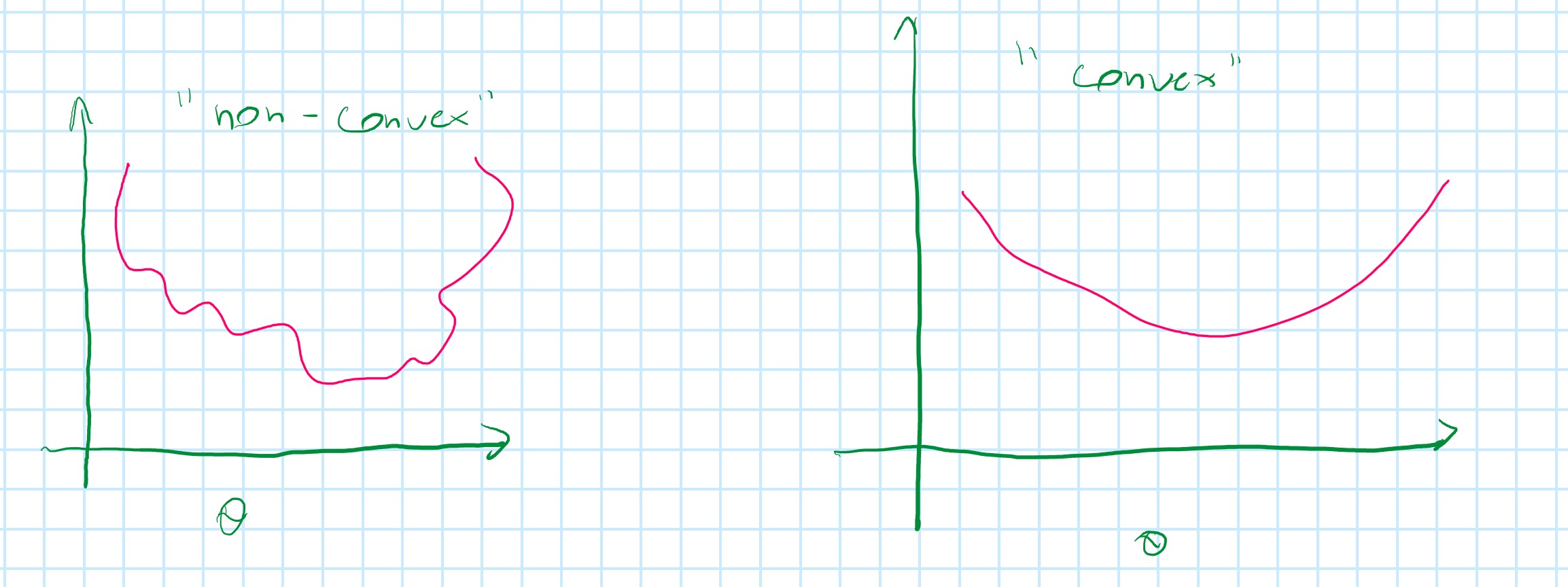
This function is fine for linear regression.

For logistic regression would also work fine, but as well would be a non-convex function of the parameters $\theta$

Example:

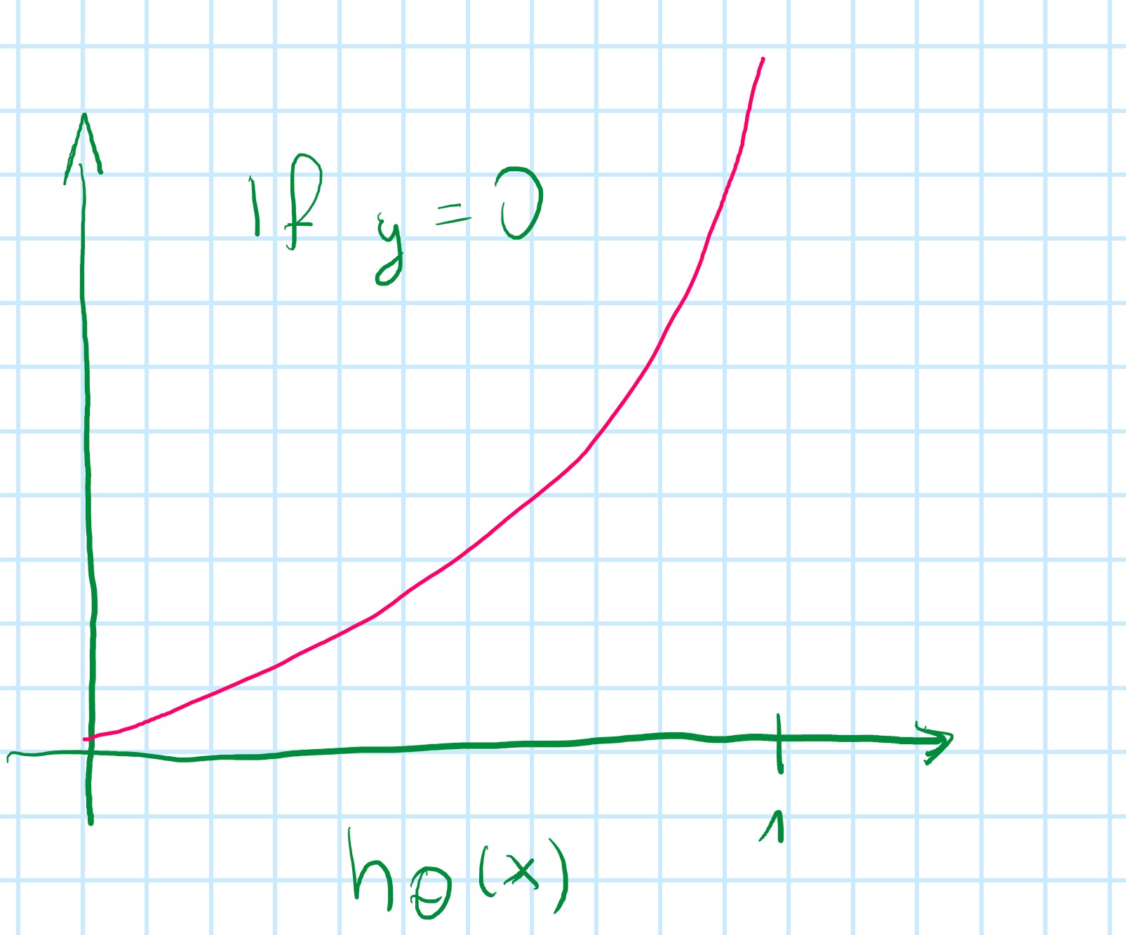
Logistic regression cost function

$Cost (h_θ (x^{(i)}) = \begin{array}{cc} \log(h_{\theta}(x)) \text{if } y = 1 \\ \log(1 - h_{\theta}(x)) \text{if } y = 0 \end{array}$

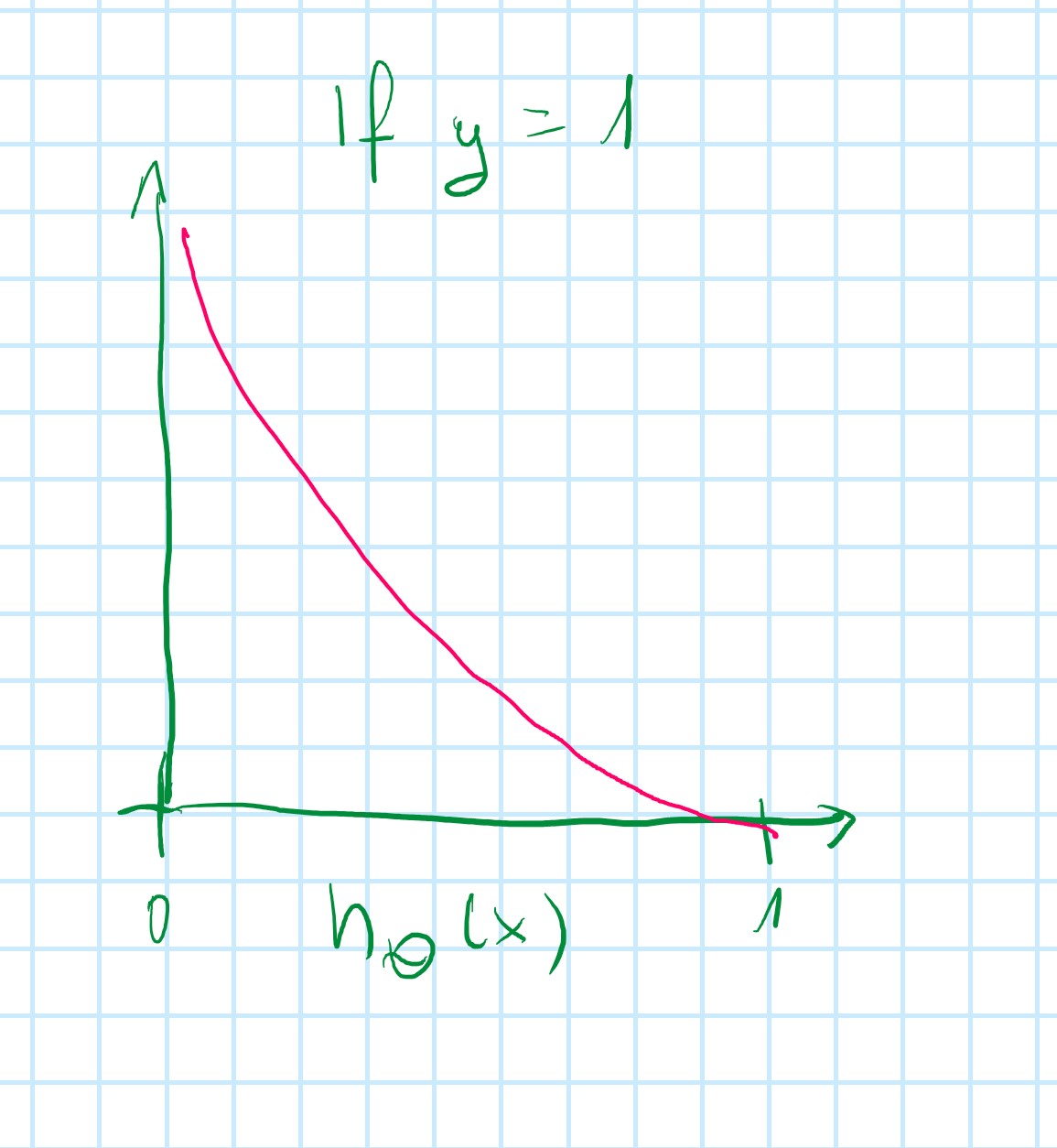
$Cost = 0$ if $y = 1, h_{\theta}(x) = 1$

But as $h_{\theta}(x) \to 0$ and $Cost \to \infty$

Capture intuition that if $h_{\theta}(x) = 0$ (predict $P(y=1|x;\theta)=0$ ), but $y = 1$ , we will penalize learning algorithm by a very large cost

Simplified cost function and gradient descent

Logistic regression cost function

$J(θ)=\frac{1}{m} \displaystyle\sum_{i=1}^m Cost (h_θ (x^{(i)}), y^{(i)})$

$Cost (h_θ (x^{(i)}) = \begin{array}{cc} \log(h_{\theta}(x)) \text{if } y = 1 \\ \log(1 - h_{\theta}(x)) \text{if } y = 0 \end{array}$

Always $y=0 \text{ or } y=1$

$Cost (h_θ (x),y) = -y\log(h_{\theta}(x)) - ((-y)\log(1-h_{\theta}(x))$ (compact way to write in one line)

if $y=1$ : $Cost (h_θ (x),y) = -\log(h_{\theta}(x))$
if $y=0$ : $Cost (h_θ (x),y) = -\log(1 - h_{\theta}(x))$

Logistic regression cost function

$J(θ)=\frac{1}{m} \displaystyle\sum_{i=1}^m Cost (h_θ (x^{(i)}), y^{(i)}) = -\frac{1}{m} \lbrack\displaystyle\sum_{i=1}^m y^{(i)} \log h_{\theta}(x^{(i)})+(1-y^{(i)})\log(1-h_{\theta}(x^{(i)})) \rbrack$ $J(θ)=\frac{1}{m} \displaystyle\sum_{i=1}^m Cost (h_θ (x^{(i)}), y^{(i)})$

To fit parameter $\theta$ : $\begin{matrix} min \\ \theta \end{matrix} J(\theta)$

To make a prediction given new $x$ :

Output $h_{\theta}(x) = \frac{1}{1 + e^{-\theta T} x}$

Gradient Descent

$J(θ)=-\frac{1}{m} \lbrack\displaystyle\sum_{i=1}^m y^{(i)} \log h_{\theta}(x^{(i)})+(1-y^{(i)})\log(1-h_{\theta}(x^{(i)})) \rbrack$

Want $min_{\theta}J(\theta)$ :

Repeat {
$θ_j := θ_j - \alpha \frac{∂}{∂θ_j} J(θ)$
}
(simultaneously update for every $\theta_j$ )

$\alpha \frac{∂}{∂θ_j} J(θ) = \frac{1}{m} \displaystyle\sum_{i=1}^m (h_θ (x^{(i)}) - y^{(i)})x_j^{(i)}$

so:

Repeat {
$θ_j := θ_j - \alpha \displaystyle\sum_{i=1}^m (h_θ (x^{(i)}) - y^{(i)})x_j^{(i)}$
}
(simultaneously update all $\theta_j$ )

$\theta$ = $\begin{bmatrix} \theta_0 \\ \theta_1 \\ \theta_2 \\ \vdots \\ \theta_n \end{bmatrix} h_{\theta}(x)=\frac{1}{1 + e^{\theta^Tx}}$

Algorithms look identical like linear regression but have a different $h_{\theta}(x)$ definition.

Advanced Optimalisation

Optimalisation algotithms

Cost function $J(\theta)$ . Want $min_{\theta}J(\theta)$ .

Given $\theta$ , we already have a code that can compute:

$J(\theta)$
$\frac{∂}{∂θ_j} J(θ)$ (for $j=0,1,...,n$ )

Gradient descent

Repeat {
$θ_j := θ_j - \alpha \frac{∂}{∂θ_j} J(θ)$
}

Other (than Gradient descent) optimasation algorithms:

Conjugate gradient
BFGS
L-BFGS

Advantages of using those algorithms:
No need to manually peek \alpha
- have inline search algorithm that automatically tries different values for the learning rate $\alpha$ , and automatically picks a good learning rate $\alpha$
- Often faster than gradient descent

Disadvantages of using those algorithms:

More complex and advanced

Example:
$\theta = \begin{bmatrix} \theta_1 \\ \theta_2 \end{bmatrix}$

$\begin{matrix} min \\ \theta \end{matrix} J(\theta) \implies \theta_1=5; \theta_2=5$

$J(\theta) = (\theta_1 - 5)^2 + (\theta_2 - 5)^2$ (cost function)

$\frac{∂}{∂θ_1}J(\theta) = 2(\theta_1-5)$

$\frac{∂}{∂θ_2}J(\theta) = 2(\theta_2-5)$

Prove in Octave:

>> options = optimset('GradObj', 'On', 'MaxIter', 100);
>> initialTheta = zeros(2,1);
>> function [jVal, gradient] = costFunction(theta)

  jVal = (theta(1)-5)^2 + (theta(2)-5)^2;
  gradient = zeros(2,1);
  gradient(1) = 2*(theta(1)-5);
  gradient(2) = 2*(theta(2)-5);
endfunction
>> [optTheta, functionValm exitFlag] = fminunc(@costFunction, initialTheta, options)
optTheta =

   5.0000
   5.0000

functionValm =    1.5777e-30
exitFlag =  1

fminunc - Advance Optimalization function in Octave

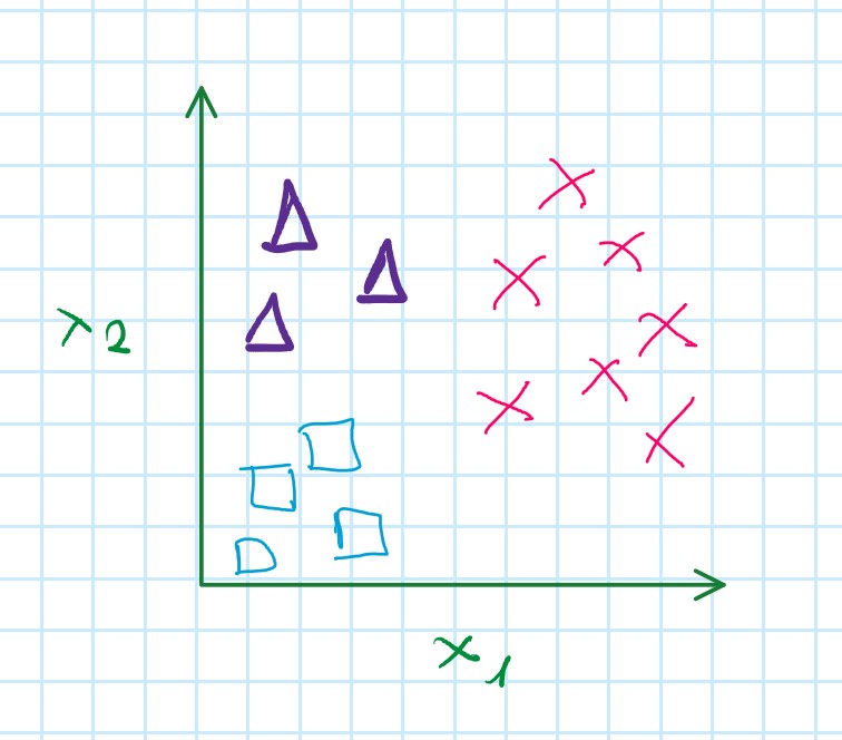
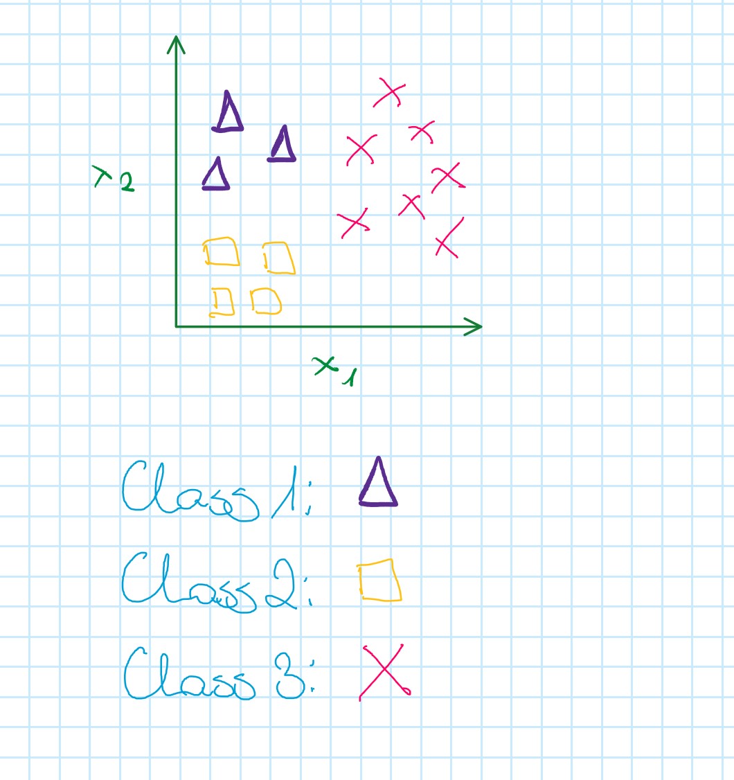
Multi-class classification: ONE-VS-ALL

Multiclass classification

Examples:

Email foldering/tagging: Work $(y=1)$ , Friends $(y=2)$ , Family $(y=3)$ , Hobby $(y=4)$
Medical diagrams: Not ill $(y=1)$ , Cold $(y=2)$ , Flu $(y=3)$
Weather: Sunny $(y=1)$ , Cloudy $(y=2)$ , Rain $(y=3)$ , Snow $(y=4)$

Binary classification

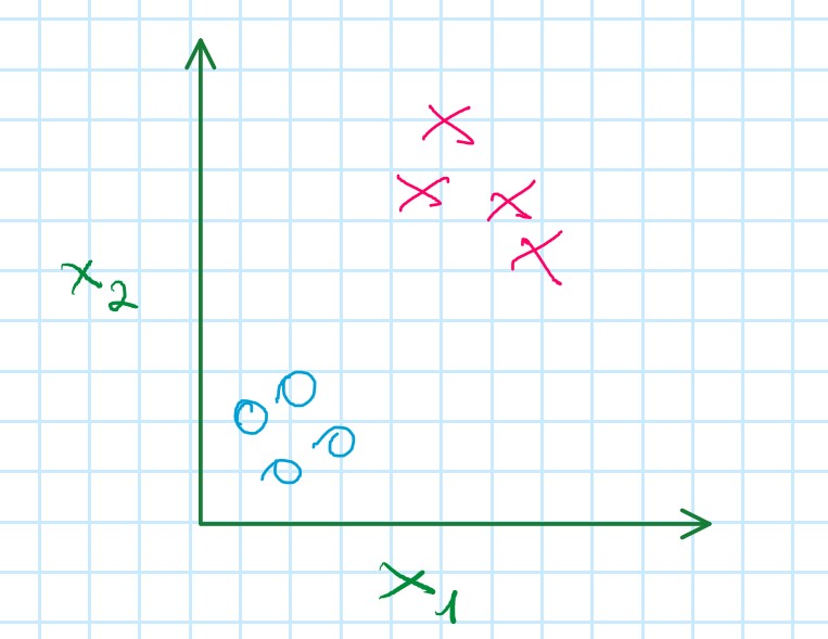
Multi-class classification

Question: How do we get a learning algorithm to work for the setting?

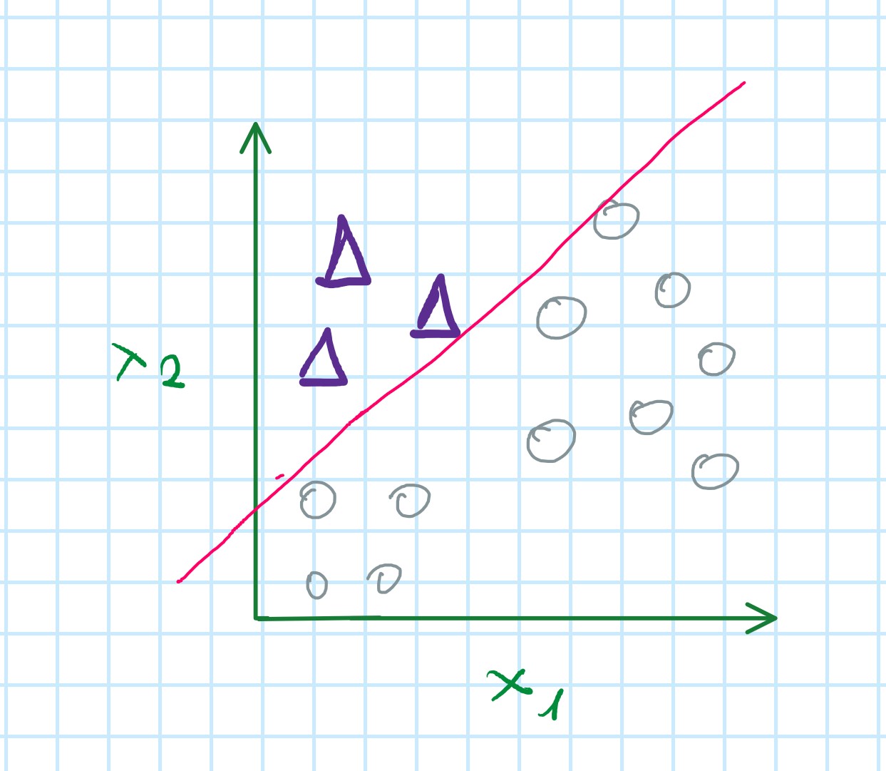
One-vs-all (one-vs-rest)

Step 1: Creating a new training set to fit the classifier $h_{\theta}^{(1)}(x)$

Step 2: Creating a new training set to fit the classifier $h_{\theta}^{(2)}(x)$

Step 3: Creating a new training set to fit the classifier $h_{\theta}^{(3)}(x)$

We fit three classifiers what is a probablity of one of the three classes:
$h_{\theta}^{(i)}(x) = P(y=i|x;\theta)$

One-vs-all

Train a logistic regression classifier $h_{\theta}^{(i)}(x)$ for each class $i$ to predict the probability that $y=i$
On a new input $x$ , to make a prediction, pick the class $i$ ythat maximaizes: $\begin{matrix} max\\ i \end{matrix} h_{\theta}^{(i)}(x)$

Cookie	Duration	Description
cookielawinfo-checkbox-analytics	11 months	This cookie is set by GDPR Cookie Consent plugin. The cookie is used to store the user consent for the cookies in the category "Analytics".
cookielawinfo-checkbox-functional	11 months	The cookie is set by GDPR cookie consent to record the user consent for the cookies in the category "Functional".
cookielawinfo-checkbox-necessary	11 months	This cookie is set by GDPR Cookie Consent plugin. The cookies is used to store the user consent for the cookies in the category "Necessary".
cookielawinfo-checkbox-others	11 months	This cookie is set by GDPR Cookie Consent plugin. The cookie is used to store the user consent for the cookies in the category "Other.
cookielawinfo-checkbox-performance	11 months	This cookie is set by GDPR Cookie Consent plugin. The cookie is used to store the user consent for the cookies in the category "Performance".
viewed_cookie_policy	11 months	The cookie is set by the GDPR Cookie Consent plugin and is used to store whether or not user has consented to the use of cookies. It does not store any personal data.

Machine Learning Coursera’s Notes – Week 3

Recent Posts

Categories

Logistic Regression

Multiclass classification problem $y \in \{0,1,2,3,...\}$

How to develop a classification algorithm?

What happens if a problem will change a bit?

Conclusion: Applying linear regression to classification problem often isn't a good idea

Logistic Regression: $0 \leqslant h_{\theta}(x) \leqslant 1$ - it's classification algorithm