My notes from the Machine Learning Course provided by Andrew Ng on Coursera

Linear Regression with Multiple Variables

Linear Regression for a single feature

h_θ(x)=θ_0+θ_1 x

Linear Regression for multiple variables

h_θ(x)=θ_0x_0+θ_1x_1+θ_2x_2+...+θ_nx_n
where x_0=1

Parameters: θ=\{θ_0,θ_1,θ_2,...,θ_n\} \in \R^{n+1}
Features: x=\{x_0,x_1,x_2,...,x_n\} \in \R^{n+1}

Notation:

• n – number of features
• x^{(i)} – input (features) of i^{th} training example
• x_j^{(i)} – values of feature j in i^{th} training example

Example:

Predict house price:

Size (feet^2)	No. of bedrooms	No. of floors	Age of house (years)	Price($1000)
\textcolor{#c91862}{x_1}	\textcolor{#c91862}{x_2}	\textcolor{#c91862}{x_3}	\textcolor{#c91862}{x_4}	\textcolor{#c91862}{h_θ(x)=y}
2104	5	1	45	460
1416	3	2	40	232
1534	3	2	30	315
852	2	1	36	178

n=4

x^{(i)}:

x^{(2)}=\begin{bmatrix} 1416 \\ 3 \\ 2 \\ 40 \end{bmatrix}
x^{(4)}=\begin{bmatrix} 852 \\ 2 \\ 1 \\ 36 \end{bmatrix}

Vector is \R^n \Rightarrow \R^4

x_j^{(i)}:
  x_1^{(2)}=1416; x_2^{(2)}=3; x_3^{(2)}=2; x_4^{(2)}=40;
  x_1^{(4)}=852; x_2^{(4)}=2; x_3^{(4)}=1; x_4^{(4)}=36;

so hypothesis function will use like below:

h_θ(x)=θ_0+2140 θ_1 + 5 θ_2 + θ_3 + 45 θ_4 = 460
h_θ(x)=θ_0+1416 θ_1 + 3 θ_2 + 2 θ_3 + 40 θ_4 = 232
h_θ(x)=θ_0+1534 θ_1 + 3 θ_2 + 2 θ_3 + 30 θ_4 = 315
h_θ(x)=θ_0+852 θ_1 + 2 θ_2 + θ_3 + 36 θ_4 = 178

Cost Function

J(θ)=\frac{1}{2m} \displaystyle\sum_{i=1}^m (h_θ (x^{(i)})-y^{(i)})^2
where
(h_θ (x^{(i)})-y^{(i)})^2 – Square Error of data i
h_θ (x^{(i)}) – Predicted value
y^{(i)} – True value

The function is called Mean Error Square (MSE)

Gradient Descent

Repeat {
  θ_j := θ_j - \alpha \frac{∂}{∂θ_j} J(θ)
}
(simultanously uptae for every j=0,...,n)

Pseudocode for gradient descent

1) n=1 (only one variable)

repeat until convergence {
  θ_0 := θ_0 - \alpha \frac{1}{m} \displaystyle\sum_{i=1}^m (h_θ (x^{(i)} )-y^{(i)})
  θ_1 := θ_1 - \alpha \frac{1}{m} \displaystyle\sum_{i=1}^m (h_θ (x^{(i)} )-y^{(i)})x^{(i)}
} simonously update θ_0, θ_1

2) n\geqslant1

repeat until convergence {
  θ_j := θ_j - \alpha \frac{1}{m} \displaystyle\sum_{i=1}^m (h_θ (x^{(i)} )-y^{(i)})x_j^{(i)}
} simonously update θ_j for j = 0,...,n

Example for more than two features

• θ_0 := θ_0 - \alpha \frac{1}{m} \displaystyle\sum_{i=1}^m (h_θ (x^{(i)} )-y^{(i)})x_0^{(i)}
    and because x_0^{(i)}=1 this pseudocode for θ_0 parameter can be written:
    θ_0 := θ_0 - \alpha \frac{1}{m} \displaystyle\sum_{i=1}^m (h_θ (x^{(i)} )-y^{(i)})
  • θ_1 := θ_1 - \alpha \frac{1}{m} \displaystyle\sum_{i=1}^m (h_θ (x^{(i)} )-y^{(i)})x_1^{(i)}
  • θ_2 := θ_2 - \alpha \frac{1}{m} \displaystyle\sum_{i=1}^m (h_θ (x^{(i)} )-y^{(i)})x_2^{(i)}

Gradient Descent in Practice

Idea: Make sure features are on a similar scale, so gradient descent coverages fast

Example:
x_1 = size (0-2000 feet^2)
x_2 = number of bedrooms (1-5)

Problem:
The x_1 have a larger range of values than x_2, so J(θ) can write very skewed elliptical shape and gradient descent on this cost function may end up with a long time of execution.

Feature Scaling

Feature scaling involves dividing the input values by the range (i.e. the maximum values minus the minimum value) of the input variable, resulting in a new range of just 1

x_1 = \frac{size(feet^2)}{2000}

x_2 = \frac{no. of bedrooms}{5}

new tange for this example:

0 \leqslant x_1 \leqslant 1
0 \leqslant x_2 \leqslant 1

The scale for the features should be approximately a \textcolor{#c91862}{-1 \leqslant x_i \leqslant 1} range

Mean Normalization

Replace x_i with x_1 - \mu_1 to make features have approximetley zero mean (don’t do for x_0=1)

Example:

x_1 = \frac{size-1000}{2000} (where average = 1000 and max=2000)
x_2 = \frac{no. of bedrooms - 2}{5} (where average = 2 and max = 5)

The new range is:
-0.5 \leqslant x_1 \leqslant 0.5
-0.5 \leqslant x_2 \leqslant 0.5

x_i = \frac{x_i-\mu_i}{s_i} where \mu_i = average of x in training set and s_i = range (max - min) or standard derivation

Learning Rate \alpha

"Debugging" – how to make sure gradient descent is working correctly.

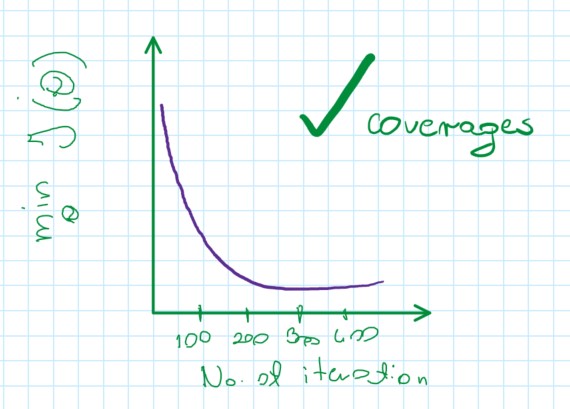
Plot min value of cost function after some number of iterations.

It’s difficult to tell how many iterations cost function need to coverage.

The function works correctly because J(\theta) decrease after each iterration:

In below example, the function is flattened and (less or more) the function is coverage as a cost function

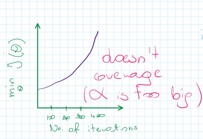
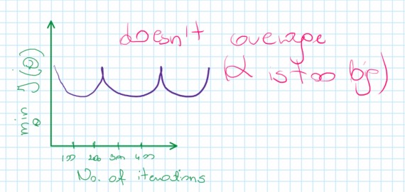
If J(\theta) increasing, probably it should use smaller \alpha

Automatic coverage test

Example: Declare coverage if J(\theta) decreases by less then the small value (10^{-3}) in one iteration.

Summary

• for sufficiently small \alpha, J(\theta) should decrease on each iteration
• if \alpha is too small: slow coverage
• if \alpha is too large: J(\theta) may not decrease on every iteration; may not coverage
• find best \alpha for speed + convergence by ploting different \alpha values, e.g. 0.01, 0.03, 0.1, 0.3...

Features and Polynomial Regression

Understanding features can allow us to create a better model e.g. by combining them:

x_1 = width
x_2 = depth
h_\theta(x)=\theta_0 + \theta_1 x_1 + \theta_2 x_2

\rightarrow combine to area

area = width * depth
x = x_1 * x_2

so

h_\theta(x) = \theta_0 + \theta_1 x (using only one feature)

Polynomial regression

Hypothesis function doesn’t need to be a straight line.

It can be polynomial by choosing features

The hypothesis function can change into quadratic, cubic or square root function (or any other form)

e.g.

hypothesis function: h_\theta(x) = \theta_0 + \theta_1 x_1

• create an additional feature based on x_1

h_\theta(x) = \theta_0 + \theta_1 x_1 + \theta_2 x_1^2 (quadratic function)
or
h_\theta(x) = \theta_0 + \theta_1 x_1 + \theta_2 x_1^2 + \theta_3 x_1^3 (cubic function)

The feature scaling is very important!

e.g. if x_1 has range 1-1000 than range of x_1^2 becomes 1-100 000 and x_1^3 becomes 1 - 100 000 000

Normal Equation

Normal equation – Method to solve \theta analytically \rightarrow finding the optimal value in just one go

Intuition: If 1D (\theta \in \R)

Cost function: J(\theta) = a\theta^2 + b\theta+c (quadratic function)

Solve for minJ(\theta) \rArr (\theta_0, \theta_1, ..., \theta_n)

• take the derivetives with respect to the \theta's and set them to 0
• \theta \in \R^{n+1} J(\theta_0,\theta_1,...,\theta_m) = \frac{1}{2m}\displaystyle\sum_{i=1}^m (h_\theta (x^{(i)})-y^{(i)})^2

\frac{\partial}{\partial \theta_j} J(\theta) = ... = 0 (for every j)

Example: m = 4 (House price prediction)

Size (feet^2)	No. of bedrooms	No. of floors	Age of house (years)	Price($1000)
\textcolor{green}{x_1}	\textcolor{green}{x_2}	\textcolor{green}{x_3}	\textcolor{green}{x_4}	\textcolor{green}{y}
2104	5	1	45	460
1416	3	2	40	232
1534	3	2	30	315
852	2	1	36	178

\Darr

Add extra column that corresponds to extra feature x that always takes value of 1

Size (feet^2)	No. of bedrooms	No. of floors	Age of house (years)	Price($1000)
\textcolor{#c91862}{x_0}	\textcolor{green}{x_1}	\textcolor{green}{x_2}	\textcolor{green}{x_3}	\textcolor{green}{x_4}	\textcolor{green}{y}
\textcolor{#c91862}{1}	2104	5	1	45	460
\textcolor{#c91862}{1}	1416	3	2	40	232
\textcolor{#c91862}{1}	1534	3	2	30	315
\textcolor{#c91862}{1}	852	2	1	36	178

so:
note
a+b+c

\underbrace{X}_{\text{features}} = \underbrace{\begin{bmatrix} 1 & 2104 & 5 & 1 & 45 \\ 1 & 1416 & 3 & 2 & 40 \\ 1 & 1534 & 3 & 2 & 30 \\ 1 & 852 & 2 & 1 & 36 \end{bmatrix}}_{\textcolor{#c91862}{\text{m x (n + 1)}}}

y = \underbrace{\begin{bmatrix} 460 \\ 232 \\ 315 \\ 178 \end{bmatrix}}_{\textcolor{#c91862}{\text{m - dimensional vector}}}

Than:

\theta = (X^TX)^{-1}X^Ty (normal equation)

In general case:

• m examples (x^{(1)}, y^{(1)}), ... , (x^{(m)}, y^{(m)})

x^{(i)} = \underbrace{\begin{bmatrix} x_0^{(i)} \\ x_1^{(i)} \\ x_2^{(i)} \\ \vdots \\ x_n^{(i)} \end{bmatrix}}_{\textcolor{#c91862}{\text{vector of all features values in the example}}} \in \R^{n+1}

Design matrix:

X = \underbrace{\begin{bmatrix} --- & (x^{(1)})^T & --- \\ --- & (x^{(2)})^T & --- \\ \vdots \\ --- & (x^{(m)})^T & --- \\ \end{bmatrix}}_{\textcolor{#c91862}{\text{m x (n + 1)}}}

E.g.

If x^{(i)} = \begin{bmatrix} 1 \\ x_1^{(i)} \end{bmatrix}
X = \begin{bmatrix} 1 & x^{(1)} \\ 1 & x_2^{(1)} \\ \vdots \\ 1 & x_m^{(1)} \end{bmatrix}
\vec{y} = \begin{bmatrix} y^{(1)} \\ y^{(2)} \\ \vdots \\ y^{(m)} \end{bmatrix}

\theta = (X^TX)^{-1}X^Ty
where:
(X^TX)^{-1} – is inverse of matrix X^TX

No need to do a feature scaling

Gradient Descent vs Normal Equation

for m training examples and n features

Gradient Descent	Normal Equation
Need to choose \alpha	No need to choose \alpha
Needs many iterations	Don’t need to iterate
\mathcal{O}(kn^2)	Need to compute (X^TX)^{-1} \Rightarrow \mathcal{O}(n^3)
Works well even when n is large	Slow if n is very large

What if X^TX is non-invertible?

Non-invertible X^TX:

• singular
• degenerate

If X^TX is non-invertible – there are usually two common causes for this:
1) Redundant features (linear dependent)

E.g. x_1 = \text{size in } feet^2
x_2 = \text{size in } m^2

2) Too many features (e.g. m \leqslant n)

delete features or use some regularization